MakeMyTrip DataScience Challenge
MakeMyTrip Data Science Hiring Challenge Problem
Given dataset contains a total of 17 columns labeled A-P, out of which A-O columns are the features and column P is the label. Column “id” specifies a unique number for every row.
Your job is to build a machine learning model to predict column P using all or some of the feature columns.
Dataset Description-
Train.csv - This file contains all the above mentioned columns. You are expected to train your models on this file.
Test.csv - This file contains all the above mentioned columns except “P” column. You have to predict this column for each records given in this file.
Importing necessary modules
import numpy as np
import pandas as pd
import matplotlib.pyplot as plt
import seaborn as sns
get_ipython().run_line_magic('matplotlib', 'inline')
import os,sys


import xgboost as xgb

from sklearn.model_selection import cross_val_score
from sklearn.preprocessing import MinMaxScaler
from sklearn import preprocessing
from sklearn.linear_model import LogisticRegression
from xgboost import XGBClassifier
from xgboost import XGBRegressor
import lightgbm as lgb
from lightgbm import LGBMRegressor
from sklearn.metrics import accuracy_score
from sklearn.model_selection import GridSearchCV
from sklearn.model_selection import StratifiedKFold
from sklearn.model_selection import train_test_split
from sklearn.metrics import matthews_corrcoef, roc_auc_score
from sklearn.model_selection import RandomizedSearchCV
#from catboost import CatBoostClassifier

#from rgf.sklearn import RGFClassifier
from sklearn.ensemble import RandomForestClassifier
from sklearn.linear_model import LogisticRegression,LinearRegression
from sklearn.linear_model import Lasso
from sklearn.linear_model import Ridge
from sklearn.preprocessing import OneHotEncoder,LabelEncoder

from sklearn.svm import SVC
from sklearn.svm import SVR
from sklearn.ensemble import ExtraTreesClassifier
from sklearn.feature_selection import VarianceThreshold

from sklearn.preprocessing import StandardScaler
from sklearn.decomposition import PCA
from sklearn.model_selection import KFold
from sklearn.metrics import r2_score
#from ggplot import *
from xgboost import XGBRegressor

import warnings
warnings.filterwarnings("ignore")


import re
from sklearn.metrics import confusion_matrix
from sklearn.metrics import accuracy_score,precision_score,recall_score,f1_score
import re
%load_ext watermark
%watermark -v -n -m -p numpy,pandas,matplotlib,seaborn,sklearn,xgboost
Wed Jan 16 2019

CPython 3.6.4
IPython 6.2.1

numpy 1.14.5
pandas 0.22.0
matplotlib 3.0.0
seaborn 0.8.1
sklearn 0.20.1
xgboost 0.7.post3

compiler   : GCC 7.2.0
system     : Linux
release    : 3.10.0-327.59.1.el7.x86_64
machine    : x86_64
processor  : x86_64
CPU cores  : 16
interpreter: 64bit
Load data into Pandas dataframe
#os.chdir('dataset')
train_df = pd.read_csv('train.csv')
test_df = pd.read_csv('test.csv')
train_df.head()
| id | A | B | C | D | E | F | G | H | I | J | K | L | M | N | O | P | |
|---|---|---|---|---|---|---|---|---|---|---|---|---|---|---|---|---|---|
| 0 | 1 | b | 18.42 | 10.415 | y | p | aa | v | 0.125 | t | f | 0 | f | g | 120.0 | 375 | 1 |
| 1 | 2 | a | 21.75 | 11.750 | u | g | c | v | 0.250 | f | f | 0 | t | g | 180.0 | 0 | 1 |
| 2 | 3 | b | 30.17 | 1.085 | y | p | c | v | 0.040 | f | f | 0 | f | g | 170.0 | 179 | 1 |
| 3 | 4 | b | 22.67 | 2.540 | y | p | c | h | 2.585 | t | f | 0 | f | g | 0.0 | 0 | 0 |
| 4 | 5 | a | 36.00 | 1.000 | u | g | c | v | 2.000 | t | t | 11 | f | g | 0.0 | 456 | 0 |
print('Train data:-\n Columns: {}  Rows: {}'.format(train_df.shape[1],train_df.shape[0]))
print('Test data:-\n Columns: {}  Rows: {}'.format(test_df.shape[1],test_df.shape[0]))
Train data:-
 Columns: 17  Rows: 552
Test data:-
 Columns: 16  Rows: 138
train_df.describe()
| id | B | C | H | K | N | O | P | |
|---|---|---|---|---|---|---|---|---|
| count | 552.000000 | 543.000000 | 552.000000 | 552.000000 | 552.000000 | 541.000000 | 552.000000 | 552.000000 |
| mean | 276.500000 | 31.364899 | 4.780136 | 2.259176 | 2.318841 | 175.162662 | 1087.576087 | 0.552536 |
| std | 159.492947 | 11.873665 | 4.938454 | 3.442564 | 4.297867 | 154.873746 | 5758.841945 | 0.497683 |
| min | 1.000000 | 13.750000 | 0.000000 | 0.000000 | 0.000000 | 0.000000 | 0.000000 | 0.000000 |
| 25% | 138.750000 | 22.500000 | 1.000000 | 0.165000 | 0.000000 | 60.000000 | 0.000000 | 0.000000 |
| 50% | 276.500000 | 28.170000 | 2.750000 | 1.000000 | 0.000000 | 152.000000 | 3.500000 | 1.000000 |
| 75% | 414.250000 | 37.665000 | 7.561250 | 2.750000 | 3.000000 | 268.000000 | 364.750000 | 1.000000 |
| max | 552.000000 | 80.250000 | 28.000000 | 28.500000 | 40.000000 | 1160.000000 | 100000.000000 | 1.000000 |
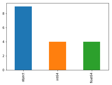
Looks like there are combination of numerical and categorical features in our dataset,lets check the countplot of column datatypes to see this.
##column datatypes barplot
train_df.dtypes.value_counts().plot(kind='bar')
<matplotlib.axes._subplots.AxesSubplot at 0x7f020d01d320>
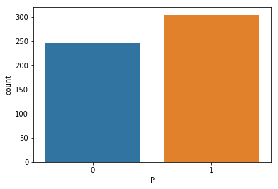
We know our target variable is ‘P’ and lets see the class distribution to identify if its skewed or balanced.
##target distribution
sns.countplot(x='P',data=train_df)
<matplotlib.axes._subplots.AxesSubplot at 0x7f020cd743c8>
categorical = list(train_df.columns[train_df.dtypes=="object"])
numerical = list(train_df.columns[train_df.dtypes!="object"])
categorical
['A', 'D', 'E', 'F', 'G', 'I', 'J', 'L', 'M']
numerical
['id', 'B', 'C', 'H', 'K', 'N', 'O', 'P']
numerical.remove('id')
numerical.remove('P')
numerical
['B', 'C', 'H', 'K', 'N', 'O']
Null counts in our numerical features
##checking for null values
print('>>>>>Numerical variables having nulls and its counts<<<<<<<<')
num_nulls = train_df[numerical].isnull().sum()[train_df[numerical].isnull().sum()>0].sort_values(ascending=False)
num_nulls
>>>>>Numerical variables having nulls and its counts<<<<<<<<


N    11
B     9
dtype: int64
Null counts in categorical features
##checking for null values
print('>>>>>Categorical variables having nulls and its counts<<<<<<<<')
cat_nulls = test_df[categorical].isnull().sum()[test_df[categorical].isnull().sum()>0].sort_values(ascending=False)
cat_nulls
>>>>>Categorical variables having nulls and its counts<<<<<<<<


A    4
G    2
F    2
E    1
D    1
dtype: int64
We’ll impute null values using median for numerical features and frequently occurring labels for categorical features.
##numerical
train_df['B'].fillna(train_df['B'].median(),inplace=True)
train_df['N'].fillna(train_df['N'].median(),inplace=True)
test_df['B'].fillna(train_df['B'].median(),inplace=True)
test_df['N'].fillna(train_df['N'].median(),inplace=True)
train_df['A'].fillna(train_df['A'].value_counts().index[0],inplace=True)
train_df['G'].fillna(train_df['G'].value_counts().index[0],inplace=True)
train_df['F'].fillna(train_df['F'].value_counts().index[0],inplace=True)
train_df['E'].fillna(train_df['E'].value_counts().index[0],inplace=True)
train_df['D'].fillna(train_df['D'].value_counts().index[0],inplace=True)

test_df['A'].fillna(train_df['A'].value_counts().index[0],inplace=True)
test_df['G'].fillna(train_df['G'].value_counts().index[0],inplace=True)
test_df['F'].fillna(train_df['F'].value_counts().index[0],inplace=True)
test_df['E'].fillna(train_df['E'].value_counts().index[0],inplace=True)
test_df['D'].fillna(train_df['D'].value_counts().index[0],inplace=True)
original_train = train_df.copy()
original_test = test_df.copy()
Exploratory Data Analysis
Distribution of Continuous Variables and Effect on Target
from scipy.stats import skew, boxcox
skewed_feats = train_df[numerical].apply(lambda x: skew(x.dropna()))
print("\nSkew in numeric features:")
print(skewed_feats)
Skew in numeric features:
B     1.124167
C     1.413447
H     2.989292
K     2.903900
N     1.373721
O    12.087691
dtype: float64
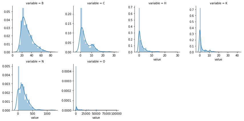
The skewness of numerical features indicates variable ‘O’ to be highly skewed compared to other variables.Lets also check whether the distribution is similar in both train and test sets to identify any Covariate shift in data.
###numerical columns histogram- Train
numdf=pd.melt(train_df,value_vars=numerical)
numgrid=sns.FacetGrid(numdf,col='variable',col_wrap=4,sharex=False,sharey=False)
numgrid=numgrid.map(sns.distplot,'value')
numgrid
<seaborn.axisgrid.FacetGrid at 0x7f020d1d37b8>
###we'll check the distribution in test to check for any covariate shift
###numerical columns histogram
numdf=pd.melt(test_df,value_vars=numerical)
numgrid=sns.FacetGrid(numdf,col='variable',col_wrap=4,sharex=False,sharey=False)
numgrid=numgrid.map(sns.distplot,'value')
numgrid
<seaborn.axisgrid.FacetGrid at 0x7f020c3c2048>
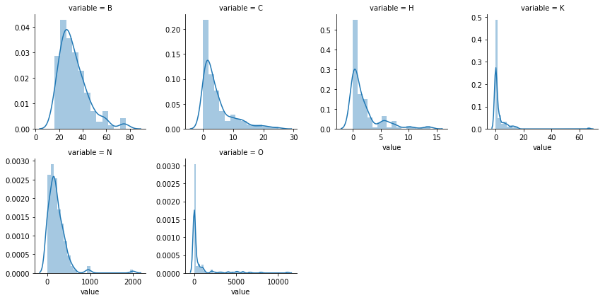
Both train and test data seems to have similar distribution and therefore no covariate shift in data.
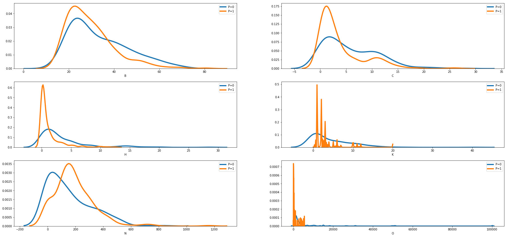
We can see how the distribution of features changes for each of the binary output variable using density plot comparing distibution for P=0 and P=1.
def density_plot(df):
    ''' Explore data by plotting KDE graphs. '''

    fig = plt.figure(1, figsize=(25,10))

    fig.subplots_adjust(bottom= -1, left=0.025, top = 2, right=0.975)
    i = 1

    for col in df.columns:
        if col=='P':
            continue
        plt.subplot(8,2,0 + i)
        j = i - 1

        #Plot KDE for all labels
        sns.distplot(df[df['P'] == 0].iloc[:,j], hist = False, label = 'P=0', kde_kws={"lw":4})
        sns.distplot(df[df['P'] == 1].iloc[:,j], hist = False, label = 'P=1', kde_kws={"lw":4})
        plt.legend();
        i = i + 1

    #Define plot format
    #DefaultSize = fig.get_size_inches()
    #fig.set_size_inches((DefaultSize[0]*1.2, DefaultSize[1]*1.2))

    plt.show()
density_plot(train_df[numerical+['P']])
##visualizing the contingency table for each categorical variable
def countplot(x,y,**kwargs):
            #sns.boxplot(x=x,y=y)
            sns.countplot(x=x,hue=y)#,data=train_df)
            #x = plt.xticks(rotation=90)


p = pd.melt(train_df, value_vars=categorical,id_vars='P')
g = sns.FacetGrid (p, col='variable', col_wrap=4, sharex=False, sharey=False, size=3)
g = g.map(countplot, 'value','P')
g.add_legend()
<seaborn.axisgrid.FacetGrid at 0x7f020caa9ef0>
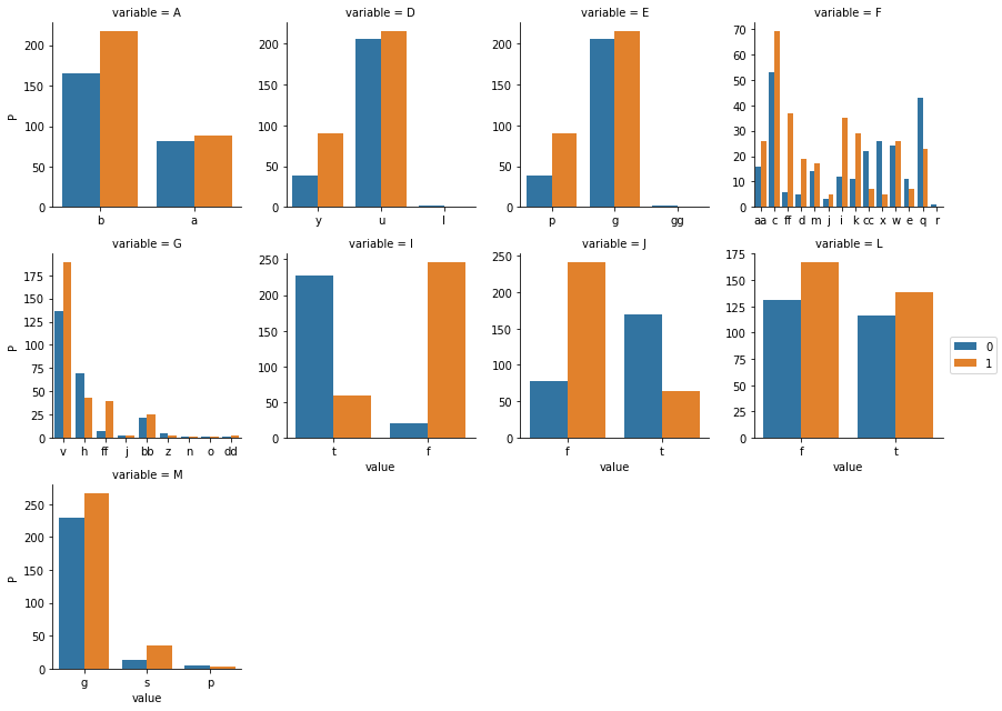
train_df['P'] = train_df['P'].astype('str')
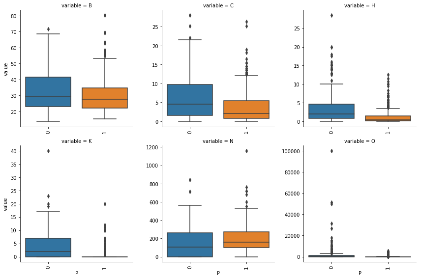
Box plots indicating the spread of numerical features for both labels of our target variable
def boxplot(x,y,**kwargs):
            sns.boxplot(x=x,y=y)
            x = plt.xticks(rotation=90)
p = pd.melt(train_df, value_vars=numerical,id_vars='P')
g = sns.FacetGrid (p, col='variable', col_wrap=3, sharex=False, sharey=False, size=4)
g = g.map(boxplot, 'P','value')
train_df[numerical].corr()
| B | C | H | K | N | O | |
|---|---|---|---|---|---|---|
| B | 1.000000 | 0.151406 | 0.404109 | 0.242301 | -0.077251 | 0.014244 |
| C | 0.151406 | 1.000000 | 0.287374 | 0.301832 | -0.208412 | 0.141069 |
| H | 0.404109 | 0.287374 | 1.000000 | 0.390157 | -0.113929 | 0.050995 |
| K | 0.242301 | 0.301832 | 0.390157 | 1.000000 | -0.164861 | 0.066033 |
| N | -0.077251 | -0.208412 | -0.113929 | -0.164861 | 1.000000 | 0.080144 |
| O | 0.014244 | 0.141069 | 0.050995 | 0.066033 | 0.080144 | 1.000000 |
Encoding Categorical features
##categorical features label encoding
from sklearn.preprocessing import LabelEncoder
le = LabelEncoder()
for col in categorical:
    le.fit(train_df[col])
    train_df[col+'_label'] = le.transform(train_df[col])
    test_df[col+'_label'] = le.transform(test_df[col])
cat_label_feat = [x for x in train_df.columns if re.search(r".*label.*",x)]
for col in cat_label_feat:
    train_df[col] = train_df[col].astype('category')
    test_df[col] = test_df[col].astype('category')
##categorical features one-hot encoding

for col in categorical:
    train_df[col] = train_df[col].astype('str')
    test_df[col] = test_df[col].astype('str')
ohencoder = OneHotEncoder(categories='auto')
for col in categorical:
    encoded = ohencoder.fit_transform(train_df[col].reshape(-1,1)).toarray()

    dfOneHot = pd.DataFrame(encoded, columns = [str(col)+'_ohe_'+str(int(i)) for i in range(encoded.shape[1])])
    train_df = pd.concat([train_df, dfOneHot], axis=1)

    encoded_test = ohencoder.transform(test_df[col].reshape(-1,1)).toarray()
    dfOneHot_test = pd.DataFrame(encoded_test, columns = [str(col)+'_ohe_'+str(int(i)) for i in range(encoded_test.shape[1])])
    test_df = pd.concat([test_df, dfOneHot_test], axis=1)
import re
ohe_feat = [x for x in train_df.columns if re.search(r".*ohe.*",x)]
for col in categorical:
    train_df[col] = train_df[col].astype('category')
    test_df[col] = test_df[col].astype('category')
train_labels  = train_df['P']
train_df  = train_df.drop(['P'],axis=1)
target = ['P']
##saving data
train_df.to_csv('trn_label_enc_ohe_enc.csv', index=False)
test_df.to_csv('tst_label_enc_ohe_enc.csv', index=False)

np.save('y_trn.npy', train_labels.values)
from sklearn.metrics import accuracy_score,precision_score,recall_score,f1_score,roc_auc_score,precision_recall_curve,log_loss
As we know our target variable is balanced and hence instead of stratified kfold cross validation we’ll perform repeated k-fold n times with different splits in each repetition using RepeatedKFold.
from sklearn.model_selection import RepeatedKFold
def repeat_kfold(train_data,feat_cols,lr):
    split = RepeatedKFold(n_splits=5,n_repeats=3,random_state=43)
    i=1
    j=1
    final_result = dict()
    for train_index,test_index in split.split(train_df):
        #print("##########")
        dict_results = dict()
        X_train , X_val = train_data.iloc[train_index],train_data.iloc[test_index]
        y_train , y_val = train_labels.iloc[train_index],train_labels.iloc[test_index]
        X_train = X_train[feat_cols]
        X_val = X_val[feat_cols]
        lr.fit(X_train,y_train)
        y_predicted_val = lr.predict_proba(X_val)[:,1]
        auc = roc_auc_score(y_val, y_predicted_val)
        dict_results['accuracy'] = accuracy_score(y_val, lr.predict(X_val))
        dict_results['precision'] = precision_score(y_val, lr.predict(X_val),pos_label="1")
        dict_results['recall'] = recall_score(y_val, lr.predict(X_val),pos_label="1")
        dict_results['f1score'] = f1_score(y_val, lr.predict(X_val),pos_label="1")
        dict_results['roc_auc_score'] = auc
        tn, fp, fn, tp = confusion_matrix(y_val, lr.predict(X_val)).ravel()
        dict_results['TN'] = tn
        dict_results['FP'] = fp
        dict_results['FN'] = fn
        dict_results['TP'] = tp
        if i%5==0:
            j+=1
            i=0

        final_result['fold'+str(i)+'_repetition'+str(j)]= dict_results
        #print(str(i)+'fold completed')
        i+=1
    return pd.DataFrame(final_result).T
Logistic Regression with Numerical and Categorical(OHE) features
##Logistic Regression
from sklearn.linear_model import LogisticRegression
lr = LogisticRegression()
#lr.fit(X_train,y_train)
result = repeat_kfold(train_df,numerical+ohe_feat,lr)
result.T
| fold0_repetition2 | fold0_repetition3 | fold0_repetition4 | fold1_repetition1 | fold1_repetition2 | fold1_repetition3 | fold2_repetition1 | fold2_repetition2 | fold2_repetition3 | fold3_repetition1 | fold3_repetition2 | fold3_repetition3 | fold4_repetition1 | fold4_repetition2 | fold4_repetition3 | |
|---|---|---|---|---|---|---|---|---|---|---|---|---|---|---|---|
| FN | 9.000000 | 12.000000 | 7.000000 | 6.000000 | 7.000000 | 3.000000 | 9.000000 | 9.000000 | 7.000000 | 12.000000 | 14.000000 | 14.000000 | 7.000000 | 7.000000 | 8.000000 |
| FP | 2.000000 | 10.000000 | 9.000000 | 18.000000 | 5.000000 | 4.000000 | 4.000000 | 7.000000 | 8.000000 | 2.000000 | 7.000000 | 4.000000 | 8.000000 | 7.000000 | 10.000000 |
| TN | 41.000000 | 36.000000 | 35.000000 | 35.000000 | 47.000000 | 51.000000 | 43.000000 | 41.000000 | 45.000000 | 46.000000 | 43.000000 | 38.000000 | 48.000000 | 44.000000 | 43.000000 |
| TP | 58.000000 | 52.000000 | 59.000000 | 52.000000 | 52.000000 | 53.000000 | 55.000000 | 54.000000 | 51.000000 | 50.000000 | 46.000000 | 54.000000 | 47.000000 | 52.000000 | 49.000000 |
| accuracy | 0.900000 | 0.800000 | 0.854545 | 0.783784 | 0.891892 | 0.936937 | 0.882883 | 0.855856 | 0.864865 | 0.872727 | 0.809091 | 0.836364 | 0.863636 | 0.872727 | 0.836364 |
| f1score | 0.913386 | 0.825397 | 0.880597 | 0.812500 | 0.896552 | 0.938053 | 0.894309 | 0.870968 | 0.871795 | 0.877193 | 0.814159 | 0.857143 | 0.862385 | 0.881356 | 0.844828 |
| precision | 0.966667 | 0.838710 | 0.867647 | 0.742857 | 0.912281 | 0.929825 | 0.932203 | 0.885246 | 0.864407 | 0.961538 | 0.867925 | 0.931034 | 0.854545 | 0.881356 | 0.830508 |
| recall | 0.865672 | 0.812500 | 0.893939 | 0.896552 | 0.881356 | 0.946429 | 0.859375 | 0.857143 | 0.879310 | 0.806452 | 0.766667 | 0.794118 | 0.870370 | 0.881356 | 0.859649 |
| roc_auc_score | 0.970149 | 0.880095 | 0.881198 | 0.852960 | 0.936441 | 0.963961 | 0.930851 | 0.933532 | 0.925179 | 0.963710 | 0.905000 | 0.933824 | 0.928241 | 0.922233 | 0.903012 |
print("mean accuracy >>",result.mean()['accuracy'])
print("mean precision >>",result.mean()['precision'])
print("mean recall >>",result.mean()['recall'])
print("mean f1score >>",result.mean()['f1score'])
print("mean roc_auc_score >>",result.mean()['roc_auc_score'])
mean accuracy >> 0.8574447174447174
mean precision >> 0.884449947598636
mean recall >> 0.8580591211653511
mean f1score >> 0.8693746677694869
mean roc_auc_score >> 0.9220257309243639
Linear Discriminant Analysis
##Linear disriminant analysis
from sklearn.discriminant_analysis import LinearDiscriminantAnalysis as LDA
train_df_scaled = train_df.copy()
test_df_scaled = test_df.copy()
sc = StandardScaler()
train_df_scaled[numerical] = sc.fit_transform(train_df_scaled[numerical])
test_df_scaled[numerical] = sc.transform(test_df_scaled[numerical])
from sklearn.model_selection import train_test_split

X_train, X_test, y_train, y_test = train_test_split(train_df_scaled[numerical+ohe_feat], train_labels, test_size=0.2, random_state=0)
##saving data
##saving data
train_df_scaled.to_csv('trn_scaled_label_enc_ohe_enc.csv', index=False)
test_df_scaled.to_csv('tst_scaled_label_enc_ohe_enc.csv', index=False)

#np.save('y_trn.npy', train_labels.values)
lda = LDA(n_components=2)
X_train = lda.fit_transform(X_train, y_train)
X_test = lda.transform(X_test)
clf = LogisticRegression(random_state = 0)
clf.fit(X_train, y_train)


y_pred = clf.predict(X_test)
print('accuracy',accuracy_score(y_test, y_pred))
print('precision',precision_score(y_test, y_pred,pos_label="1"))
print('recall',recall_score(y_test, y_pred,pos_label="1"))
print('f1_score',f1_score(y_test, y_pred,pos_label="1"))
accuracy 0.8468468468468469
precision 0.9491525423728814
recall 0.8
f1_score 0.8682170542635659
Since we are dealing with balanced target class, LDA is able to perform well and approximates the bayes classifier decision boundary.
Random Forest Classifier
##RandomForest Classifier
from sklearn.ensemble import RandomForestClassifier
rf_clf = RandomForestClassifier(random_state=43)
#result_rf = repeat_kfold(train_df,rf_clf)
n_estimators = [int(x) for x in np.linspace(start = 200, stop = 2000, num = 10)]# Number of trees in random forest
max_features = ['auto', 'sqrt']# Number of features to consider at every split
max_depth = [int(x) for x in np.linspace(10, 110, num = 11)]# Maximum number of levels in tree
max_depth.append(None)
min_samples_split = [2, 5, 10]# Minimum number of samples required to split a node
min_samples_leaf = [1, 2, 4]# Minimum number of samples required at each leaf node
bootstrap = [True, False]# Method of selecting samples for training each tree
# Create the random grid
rf_param_grid = {'n_estimators': n_estimators,
               'max_features': max_features,
               'max_depth': max_depth,
               'min_samples_split': min_samples_split,
               'min_samples_leaf': min_samples_leaf,
               'bootstrap': bootstrap}
clf_random = RandomizedSearchCV(estimator = rf_clf,scoring='roc_auc', param_distributions = rf_param_grid, n_iter = 100, cv = 3, verbose=2, random_state=42, n_jobs = -1)

clf_random.fit(train_df[numerical+ohe_feat], train_labels)
Fitting 3 folds for each of 100 candidates, totalling 300 fits


[Parallel(n_jobs=-1)]: Using backend LokyBackend with 16 concurrent workers.
[Parallel(n_jobs=-1)]: Done   9 tasks      | elapsed:    5.8s
[Parallel(n_jobs=-1)]: Done 130 tasks      | elapsed:   25.1s
[Parallel(n_jobs=-1)]: Done 300 out of 300 | elapsed:   55.0s finished


RandomizedSearchCV(cv=3, error_score='raise-deprecating',
          estimator=RandomForestClassifier(bootstrap=True, class_weight=None, criterion='gini',
            max_depth=None, max_features='auto', max_leaf_nodes=None,
            min_impurity_decrease=0.0, min_impurity_split=None,
            min_samples_leaf=1, min_samples_split=2,
            min_weight_fraction_leaf=0.0, n_estimators='warn', n_jobs=None,
            oob_score=False, random_state=43, verbose=0, warm_start=False),
          fit_params=None, iid='warn', n_iter=100, n_jobs=-1,
          param_distributions={'n_estimators': [200, 400, 600, 800, 1000, 1200, 1400, 1600, 1800, 2000], 'max_features': ['auto', 'sqrt'], 'max_depth': [10, 20, 30, 40, 50, 60, 70, 80, 90, 100, 110, None], 'min_samples_split': [2, 5, 10], 'min_samples_leaf': [1, 2, 4], 'bootstrap': [True, False]},
          pre_dispatch='2*n_jobs', random_state=42, refit=True,
          return_train_score='warn', scoring='roc_auc', verbose=2)
clf_random.best_params_
{'bootstrap': True,
 'max_depth': 80,
 'max_features': 'auto',
 'min_samples_leaf': 1,
 'min_samples_split': 5,
 'n_estimators': 600}
result_rf = repeat_kfold(train_df,numerical+ohe_feat,clf_random.best_estimator_)
print("mean accuracy >>",result_rf.mean()['accuracy'])
print("mean precision >>",result_rf.mean()['precision'])
print("mean recall >>",result_rf.mean()['recall'])
print("mean f1score >>",result_rf.mean()['f1score'])
print("mean roc_auc_score >>",result_rf.mean()['roc_auc_score'])
mean accuracy >> 0.8659022659022659
mean precision >> 0.883079819082217
mean recall >> 0.8764090885530088
mean f1score >> 0.8782733325932504
mean roc_auc_score >> 0.9361335877218927
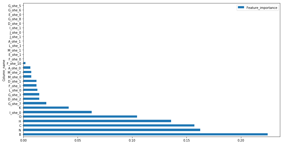
feat_imp = pd.DataFrame(clf_random.best_estimator_.feature_importances_)
feat_imp.columns = ['Feature_importance']
feat_imp = feat_imp.assign(Column_name=numerical+ohe_feat)
feat_imp.sort_values(by=['Feature_importance'],ascending=False).set_index('Column_name').head(30).plot(kind='barh',figsize=(15,8))
<matplotlib.axes._subplots.AxesSubplot at 0x7f0204377208>
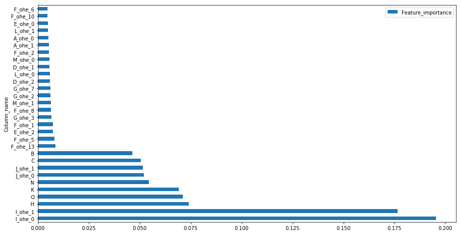
The importance of feature I and J with low cardinalty is evident from the contingency plots of variable classes with the target value plotted above and it has been considered important in tree building process for splits whereas high cardinal features have less importance
XGBOOST
##XGBOOST
from xgboost import XGBClassifier
xgb_model = XGBClassifier()
param_dist = {"max_depth": [10,30,50],
              "min_child_weight" : [1,3,6],
              "n_estimators": [200],
              "learning_rate": [0.05, 0.1,0.16],}
grid_search = GridSearchCV(xgb_model, param_grid=param_dist, cv = 3,
                                   verbose=10, n_jobs=-1)
grid_search.fit(train_df[numerical+ohe_feat],train_labels)
Fitting 3 folds for each of 27 candidates, totalling 81 fits


[Parallel(n_jobs=-1)]: Using backend LokyBackend with 16 concurrent workers.
[Parallel(n_jobs=-1)]: Done   9 tasks      | elapsed:    0.5s
[Parallel(n_jobs=-1)]: Done  18 tasks      | elapsed:    0.6s
[Parallel(n_jobs=-1)]: Done  29 tasks      | elapsed:    0.8s
[Parallel(n_jobs=-1)]: Done  40 tasks      | elapsed:    1.1s
[Parallel(n_jobs=-1)]: Done  59 out of  81 | elapsed:    1.4s remaining:    0.5s
[Parallel(n_jobs=-1)]: Done  68 out of  81 | elapsed:    1.5s remaining:    0.3s
[Parallel(n_jobs=-1)]: Done  77 out of  81 | elapsed:    1.6s remaining:    0.1s
[Parallel(n_jobs=-1)]: Done  81 out of  81 | elapsed:    1.7s finished


GridSearchCV(cv=3, error_score='raise-deprecating',
       estimator=XGBClassifier(base_score=0.5, booster='gbtree', colsample_bylevel=1,
       colsample_bytree=1, gamma=0, learning_rate=0.1, max_delta_step=0,
       max_depth=3, min_child_weight=1, missing=None, n_estimators=100,
       n_jobs=1, nthread=None, objective='binary:logistic', random_state=0,
       reg_alpha=0, reg_lambda=1, scale_pos_weight=1, seed=None,
       silent=True, subsample=1),
       fit_params=None, iid='warn', n_jobs=-1,
       param_grid={'max_depth': [10, 30, 50], 'min_child_weight': [1, 3, 6], 'n_estimators': [200], 'learning_rate': [0.05, 0.1, 0.16]},
       pre_dispatch='2*n_jobs', refit=True, return_train_score='warn',
       scoring=None, verbose=10)
grid_search.best_estimator_
XGBClassifier(base_score=0.5, booster='gbtree', colsample_bylevel=1,
       colsample_bytree=1, gamma=0, learning_rate=0.16, max_delta_step=0,
       max_depth=10, min_child_weight=3, missing=None, n_estimators=200,
       n_jobs=1, nthread=None, objective='binary:logistic', random_state=0,
       reg_alpha=0, reg_lambda=1, scale_pos_weight=1, seed=None,
       silent=True, subsample=1)
grid_search.best_params_
{'learning_rate': 0.16,
 'max_depth': 10,
 'min_child_weight': 3,
 'n_estimators': 200}
final_xgb = XGBClassifier(max_depth=10, min_child_weight=3,  n_estimators=200,\
                          n_jobs=-1 , verbose=1,learning_rate=0.16)
result_xgb = repeat_kfold(train_df,numerical+ohe_feat,final_xgb)
result_xgb.T
| fold0_repetition2 | fold0_repetition3 | fold0_repetition4 | fold1_repetition1 | fold1_repetition2 | fold1_repetition3 | fold2_repetition1 | fold2_repetition2 | fold2_repetition3 | fold3_repetition1 | fold3_repetition2 | fold3_repetition3 | fold4_repetition1 | fold4_repetition2 | fold4_repetition3 | |
|---|---|---|---|---|---|---|---|---|---|---|---|---|---|---|---|
| FN | 10.000000 | 6.000000 | 7.000000 | 7.000000 | 6.000000 | 5.000000 | 6.000000 | 6.000000 | 5.000000 | 8.000000 | 11.000000 | 12.000000 | 5.000000 | 7.000000 | 7.000000 |
| FP | 2.000000 | 10.000000 | 6.000000 | 13.000000 | 5.000000 | 8.000000 | 12.000000 | 4.000000 | 9.000000 | 3.000000 | 5.000000 | 6.000000 | 8.000000 | 6.000000 | 10.000000 |
| TN | 41.000000 | 36.000000 | 38.000000 | 40.000000 | 47.000000 | 47.000000 | 35.000000 | 44.000000 | 44.000000 | 45.000000 | 45.000000 | 36.000000 | 48.000000 | 45.000000 | 43.000000 |
| TP | 57.000000 | 58.000000 | 59.000000 | 51.000000 | 53.000000 | 51.000000 | 58.000000 | 57.000000 | 53.000000 | 54.000000 | 49.000000 | 56.000000 | 49.000000 | 52.000000 | 50.000000 |
| accuracy | 0.890909 | 0.854545 | 0.881818 | 0.819820 | 0.900901 | 0.882883 | 0.837838 | 0.909910 | 0.873874 | 0.900000 | 0.854545 | 0.836364 | 0.881818 | 0.881818 | 0.845455 |
| f1score | 0.904762 | 0.878788 | 0.900763 | 0.836066 | 0.905983 | 0.886957 | 0.865672 | 0.919355 | 0.883333 | 0.907563 | 0.859649 | 0.861538 | 0.882883 | 0.888889 | 0.854701 |
| precision | 0.966102 | 0.852941 | 0.907692 | 0.796875 | 0.913793 | 0.864407 | 0.828571 | 0.934426 | 0.854839 | 0.947368 | 0.907407 | 0.903226 | 0.859649 | 0.896552 | 0.833333 |
| recall | 0.850746 | 0.906250 | 0.893939 | 0.879310 | 0.898305 | 0.910714 | 0.906250 | 0.904762 | 0.913793 | 0.870968 | 0.816667 | 0.823529 | 0.907407 | 0.881356 | 0.877193 |
| roc_auc_score | 0.962513 | 0.891304 | 0.907713 | 0.885491 | 0.947197 | 0.950974 | 0.941157 | 0.957011 | 0.936239 | 0.950941 | 0.919333 | 0.937325 | 0.928241 | 0.941841 | 0.926514 |
print("mean accuracy >>",result_xgb.mean()['accuracy'])
print("mean precision >>",result_xgb.mean()['precision'])
print("mean recall >>",result_xgb.mean()['recall'])
print("mean f1score >>",result_xgb.mean()['f1score'])
print("mean roc_auc_score >>",result_xgb.mean()['roc_auc_score'])
mean accuracy >> 0.8701665301665302
mean precision >> 0.8844788163422947
mean recall >> 0.8827460352351812
mean f1score >> 0.882460079578879
mean roc_auc_score >> 0.9322530204921271
feat_imp = pd.DataFrame(final_xgb.feature_importances_)
feat_imp.columns = ['Feature_importance']
feat_imp = feat_imp.assign(Column_name=numerical+ohe_feat)
feat_imp.sort_values(by=['Feature_importance'],ascending=False).set_index('Column_name').head(30).plot(kind='barh',figsize=(15,8))
<matplotlib.axes._subplots.AxesSubplot at 0x7f02042c5c50>
LightGBM
##Lightgbm
import lightgbm as lgb

lg = lgb.LGBMClassifier(silent=False)
param_dist = {"max_depth": [25,50, 75],
              "learning_rate" : [0.01,0.05,0.1],
              "num_leaves": [300,900,1200],
              "n_estimators": [200]
             }
grid_search = GridSearchCV(lg, n_jobs=-1, param_grid=param_dist, cv = 3, scoring="roc_auc", verbose=5)
grid_search.fit(train_df[numerical+categorical],train_labels)
Fitting 3 folds for each of 27 candidates, totalling 81 fits


[Parallel(n_jobs=-1)]: Using backend LokyBackend with 16 concurrent workers.
[Parallel(n_jobs=-1)]: Done  40 tasks      | elapsed:    0.9s
[Parallel(n_jobs=-1)]: Done  67 out of  81 | elapsed:    1.4s remaining:    0.3s
[Parallel(n_jobs=-1)]: Done  81 out of  81 | elapsed:    1.6s finished


GridSearchCV(cv=3, error_score='raise-deprecating',
       estimator=LGBMClassifier(boosting_type='gbdt', class_weight=None, colsample_bytree=1.0,
        learning_rate=0.1, max_depth=-1, min_child_samples=20,
        min_child_weight=0.001, min_split_gain=0.0, n_estimators=100,
        n_jobs=-1, num_leaves=31, objective=None, random_state=None,
        reg_alpha=0.0, reg_lambda=0.0, silent=False, subsample=1.0,
        subsample_for_bin=200000, subsample_freq=1),
       fit_params=None, iid='warn', n_jobs=-1,
       param_grid={'max_depth': [25, 50, 75], 'learning_rate': [0.01, 0.05, 0.1], 'num_leaves': [300, 900, 1200], 'n_estimators': [200]},
       pre_dispatch='2*n_jobs', refit=True, return_train_score='warn',
       scoring='roc_auc', verbose=5)
lgbm_params = grid_search.best_params_
lgbm_params
{'learning_rate': 0.05,
 'max_depth': 25,
 'n_estimators': 200,
 'num_leaves': 300}
###lgbm handles categorical values as-is if they are encoded as categorical type in pandas df
final_lgbm = lgb.LGBMClassifier(**lgbm_params)
result_lgbm = repeat_kfold(train_df,numerical+cat_label_feat,final_lgbm)
result_lgbm.T
| fold0_repetition2 | fold0_repetition3 | fold0_repetition4 | fold1_repetition1 | fold1_repetition2 | fold1_repetition3 | fold2_repetition1 | fold2_repetition2 | fold2_repetition3 | fold3_repetition1 | fold3_repetition2 | fold3_repetition3 | fold4_repetition1 | fold4_repetition2 | fold4_repetition3 | |
|---|---|---|---|---|---|---|---|---|---|---|---|---|---|---|---|
| FN | 9.000000 | 6.000000 | 8.000000 | 9.000000 | 7.000000 | 3.000000 | 5.000000 | 8.000000 | 4.000000 | 10.000000 | 9.000000 | 14.000000 | 2.000000 | 6.000000 | 6.000000 |
| FP | 3.000000 | 12.000000 | 9.000000 | 15.000000 | 5.000000 | 9.000000 | 9.000000 | 7.000000 | 10.000000 | 4.000000 | 7.000000 | 5.000000 | 10.000000 | 9.000000 | 8.000000 |
| TN | 40.000000 | 34.000000 | 35.000000 | 38.000000 | 47.000000 | 46.000000 | 38.000000 | 41.000000 | 43.000000 | 44.000000 | 43.000000 | 37.000000 | 46.000000 | 42.000000 | 45.000000 |
| TP | 58.000000 | 58.000000 | 58.000000 | 49.000000 | 52.000000 | 53.000000 | 59.000000 | 55.000000 | 54.000000 | 52.000000 | 51.000000 | 54.000000 | 52.000000 | 53.000000 | 51.000000 |
| accuracy | 0.890909 | 0.836364 | 0.845455 | 0.783784 | 0.891892 | 0.891892 | 0.873874 | 0.864865 | 0.873874 | 0.872727 | 0.854545 | 0.827273 | 0.890909 | 0.863636 | 0.872727 |
| f1score | 0.906250 | 0.865672 | 0.872180 | 0.803279 | 0.896552 | 0.898305 | 0.893939 | 0.880000 | 0.885246 | 0.881356 | 0.864407 | 0.850394 | 0.896552 | 0.876033 | 0.879310 |
| precision | 0.950820 | 0.828571 | 0.865672 | 0.765625 | 0.912281 | 0.854839 | 0.867647 | 0.887097 | 0.843750 | 0.928571 | 0.879310 | 0.915254 | 0.838710 | 0.854839 | 0.864407 |
| recall | 0.865672 | 0.906250 | 0.878788 | 0.844828 | 0.881356 | 0.946429 | 0.921875 | 0.873016 | 0.931034 | 0.838710 | 0.850000 | 0.794118 | 0.962963 | 0.898305 | 0.894737 |
| roc_auc_score | 0.954877 | 0.891304 | 0.915289 | 0.871828 | 0.949153 | 0.947078 | 0.952793 | 0.952712 | 0.941444 | 0.944556 | 0.926000 | 0.947479 | 0.949735 | 0.938185 | 0.934790 |
print("mean accuracy >>",result_lgbm.mean()['accuracy'])
print("mean precision >>",result_lgbm.mean()['precision'])
print("mean recall >>",result_lgbm.mean()['recall'])
print("mean f1score >>",result_lgbm.mean()['f1score'])
print("mean roc_auc_score >>",result_lgbm.mean()['roc_auc_score'])
mean accuracy >> 0.8623150423150424
mean precision >> 0.870492810959163
mean recall >> 0.8858719453656295
mean f1score >> 0.8766316283582967
mean roc_auc_score >> 0.9344815860711685
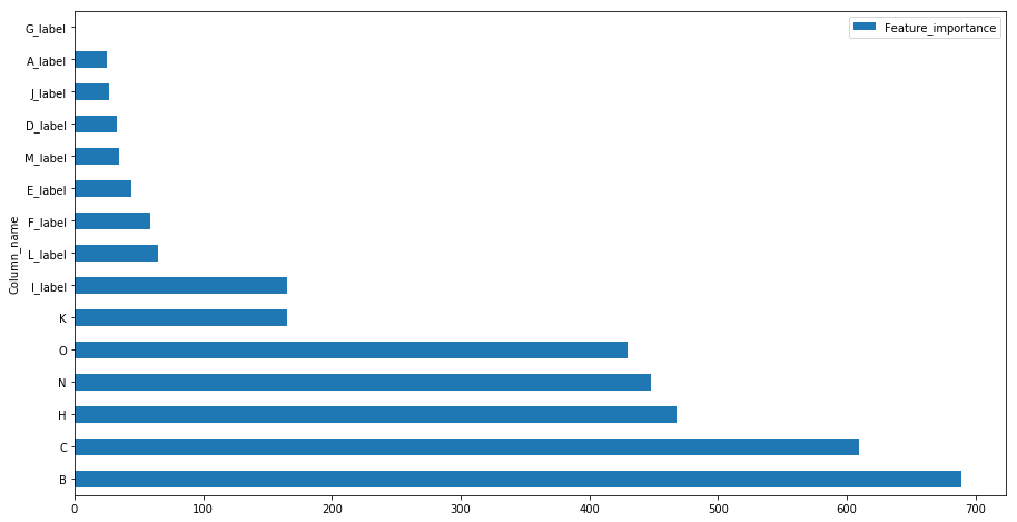
feat_imp = pd.DataFrame(final_lgbm.feature_importances_)
feat_imp.columns = ['Feature_importance']
feat_imp = feat_imp.assign(Column_name=numerical+cat_label_feat)
feat_imp.sort_values(by=['Feature_importance'],ascending=False).set_index('Column_name').head(30).plot(kind='barh',figsize=(15,8))
<matplotlib.axes._subplots.AxesSubplot at 0x7f0204219ac8>
categorical
['A', 'D', 'E', 'F', 'G', 'I', 'J', 'L', 'M']
Support Vector Classifier
##SVM
from sklearn.svm import SVC
from sklearn.model_selection import GridSearchCV

svclassifier = SVC()
param_grid_svc = {'kernel':['linear','rbf'],'C':[0.001, 0.01, 0.1, 1, 10],'gamma':[0.001, 0.01, 0.1, 1]}
svc_grid_search = GridSearchCV(estimator=svclassifier,param_grid=param_grid_svc,cv=5)
##since svm requires scaled features we'll use the scaled version of the data
svc_grid_search.fit(train_df_scaled[numerical+ohe_feat],train_labels)
GridSearchCV(cv=5, error_score='raise-deprecating',
       estimator=SVC(C=1.0, cache_size=200, class_weight=None, coef0=0.0,
  decision_function_shape='ovr', degree=3, gamma='auto_deprecated',
  kernel='rbf', max_iter=-1, probability=False, random_state=None,
  shrinking=True, tol=0.001, verbose=False),
       fit_params=None, iid='warn', n_jobs=None,
       param_grid={'kernel': ['linear', 'rbf'], 'C': [0.001, 0.01, 0.1, 1, 10], 'gamma': [0.001, 0.01, 0.1, 1]},
       pre_dispatch='2*n_jobs', refit=True, return_train_score='warn',
       scoring=None, verbose=0)
svc_grid_search.best_params_
{'C': 0.01, 'gamma': 0.001, 'kernel': 'linear'}
p = {'C': 0.01, 'gamma': 0.001, 'kernel': 'linear'}
svc_check = SVC(**p)
svc_check
SVC(C=0.01, cache_size=200, class_weight=None, coef0=0.0,
  decision_function_shape='ovr', degree=3, gamma=0.001, kernel='linear',
  max_iter=-1, probability=False, random_state=None, shrinking=True,
  tol=0.001, verbose=False)
scores = cross_val_score(svc_check,train_df_scaled[numerical+ohe_feat],train_labels,cv=3,scoring='roc_auc')
scores.mean()
0.9215289975523974
Feature engineering and transformations
We’ll perform further feature engineering techniques such as interaction features,count/frequency/mean encoding,target encoding
https://github.com/MaxHalford/xam/blob/master/docs/feature-extraction.md#smooth-target-encoding
train_df2 = train_df.copy()
test_df2 = test_df.copy()

train_df2['P'] = train_labels
for col in cat_label_feat:
    train_df2[col] = train_df2[col].astype('category').cat.codes
    test_df2[col] = test_df2[col].astype('category').cat.codes
Frequency encoding of categorical features
##frequency encoding
for col in cat_label_feat:
    encoding = train_df2.groupby(col).size()
    # get frequency of each category
    encoding = encoding/len(train_df2)
    train_df2[col+'freq_enc'] = train_df2[col].map(encoding)
    test_df2[col+'freq_enc'] = test_df2[col].map(encoding)
enc_freq_cols = [x for x in train_df2.columns if re.search(r".*freq_enc.*",x)]
Target Encoding of categorical features
def target_encoder_regularized(train, test, cols_encode, target_cols, folds = 5, stratified=True):
    """
    Mean regularized target encoding based on kfold
    """

    if stratified:
        skf = StratifiedKFold(n_splits=folds, shuffle=True, random_state=1)
        X = train.drop('P', axis=1)
        Y = train['P']
        splitter = skf.split(X, Y)
    else:
        kf = KFold(n_splits=folds, shuffle=True, random_state=1)
        splitter = kf.split(X)

    train_new = pd.DataFrame()
    for train_index, val_index in splitter:
        train_fold = train.loc[train_index]
        test_fold = train.loc[val_index]

        for by in cols_encode:
            for target in target_cols:

                encoding = train_fold.groupby(by)[target].mean()
                test_fold[target + '_mean_' + by] = test_fold[by].map(encoding)

                impute = np.mean(train_fold[target])
                test_fold.fillna(impute, inplace=True)
        train_new = pd.concat((train_new, test_fold), axis=0)

    #making test encoding using full training data
    test_new = test.copy()
    for by in cols_encode:
        for target in target_cols:
            test_new['%s_mean_%s' % (target, by)] = test_new[by].map(train_new.reset_index(drop=True).groupby(by)[target].mean())

    return train_new.reset_index(drop=True), test_new.reset_index(drop=True)
train_df2['P'] = train_df2['P'].astype('category').cat.codes
train_enc, test_enc = target_encoder_regularized(train_df2[numerical+enc_freq_cols+ohe_feat+cat_label_feat+['P']], test_df2[numerical+enc_freq_cols+ohe_feat+cat_label_feat],cat_label_feat,'P',folds = 5)
Interaction terms of all numerical features
###Interaction terms
numerics = train_enc.loc[:, numerical]
##we'll add 1 to each column values to ensure division by zero is avoided
for col in numerical:
    numerics[col] = numerics[col]+1
# for each pair of variables, determine which mathmatical operators to use based on redundancy
for i in range(0, numerics.columns.size-1):
    for j in range(0, numerics.columns.size-1):
        col1 = str(numerics.columns.values[i])
        col2 = str(numerics.columns.values[j])
        # multiply fields together (we allow values to be squared)
        if i <= j:
            name = col1 + "*" + col2
            train_enc = pd.concat([train_enc, pd.Series(numerics.iloc[:,i] * numerics.iloc[:,j], name=name)], axis=1)
        # add fields together
        if i < j:
            name = col1 + "+" + col2
            train_enc = pd.concat([train_enc, pd.Series(numerics.iloc[:,i] + numerics.iloc[:,j], name=name)], axis=1)
        # divide and subtract fields from each other
        if not i == j:
            name = col1 + "/" + col2
            train_enc = pd.concat([train_enc, pd.Series(numerics.iloc[:,i] / numerics.iloc[:,j], name=name)], axis=1)
            name = col1 + "-" + col2
            train_enc = pd.concat([train_enc, pd.Series(numerics.iloc[:,i] - numerics.iloc[:,j], name=name)], axis=1)
train_enc[feat_interact].isnull().sum()[train_enc[feat_interact].isnull().sum()>0]
Series([], dtype: int64)
###Interaction terms
numerics = test_enc.loc[:, numerical]
##we'll add 1 to each column values to ensure division by zero is avoided
for col in numerical:
    numerics[col] = numerics[col]+1
# for each pair of variables, determine which mathmatical operators to use based on redundancy
for i in range(0, numerics.columns.size-1):
    for j in range(0, numerics.columns.size-1):
        col1 = str(numerics.columns.values[i])
        col2 = str(numerics.columns.values[j])
        # multiply fields together (we allow values to be squared)
        if i <= j:
            name = col1 + "*" + col2
            test_enc = pd.concat([test_enc, pd.Series(numerics.iloc[:,i] * numerics.iloc[:,j], name=name)], axis=1)
        # add fields together
        if i < j:
            name = col1 + "+" + col2
            test_enc = pd.concat([test_enc, pd.Series(numerics.iloc[:,i] + numerics.iloc[:,j], name=name)], axis=1)
        # divide and subtract fields from each other
        if not i == j:
            name = col1 + "/" + col2
            test_enc = pd.concat([test_enc, pd.Series(numerics.iloc[:,i] / numerics.iloc[:,j], name=name)], axis=1)
            name = col1 + "-" + col2
            test_enc = pd.concat([test_enc, pd.Series(numerics.iloc[:,i] - numerics.iloc[:,j], name=name)], axis=1)
##saving data
train_enc.to_csv('trn_tgt_enc_freq_enc_label_enc_ohe_enc_interaction.csv', index=False)
test_enc.to_csv('tst_tgt_enc_freq_enc_label_enc_ohe_enc_interaction.csv', index=False)

#np.save('y_trn.npy', train_labels.values)
We’ll use (+ ,- , *, /) interaction features between all our numerical features and perform feature selection of all these.
feat_interact = ['B*C',
 'B+C',
 'B/C',
 'B-C',
 'B*H',
 'B+H',
 'B/H',
 'B-H',
 'B*K',
 'B+K',
 'B/K',
 'B-K',
 'B*N',
 'B+N',
 'B/N',
 'B-N',
 'C/B',
 'C-B',
 'C*H',
 'C+H',
 'C/H',
 'C-H',
 'C*K',
 'C+K',
 'C/K',
 'C-K',
 'C*N',
 'C+N',
 'C/N',
 'C-N',
 'H/B',
 'H-B',
 'H/C',
 'H-C',
 'H*K',
 'H+K',
 'H/K',
 'H-K',
 'H*N',
 'H+N',
 'H/N',
 'H-N',
 'K/B',
 'K-B',
 'K/C',
 'K-C',
 'K/H',
 'K-H',
 'K*N',
 'K+N',
 'K/N',
 'K-N',
 'N/B',
 'N-B',
 'N/C',
 'N-C',
 'N/H',
 'N-H',
 'N/K',
 'N-K']
enc_mean_cat = [x for x in train_enc.columns if re.search(r".*mean.*",x)]
##features selection for interaction features
feat_rf = RandomForestClassifier()
grid_feat_rf = RandomizedSearchCV(feat_rf,param_distributions=rf_param_grid,cv=5,verbose=10,n_jobs=-1)
grid_feat_rf.fit(train_enc[feat_interact],train_enc['P'])
Fitting 5 folds for each of 10 candidates, totalling 50 fits


[Parallel(n_jobs=-1)]: Using backend LokyBackend with 16 concurrent workers.
[Parallel(n_jobs=-1)]: Done   9 tasks      | elapsed:    6.2s
[Parallel(n_jobs=-1)]: Done  18 tasks      | elapsed:    7.7s
[Parallel(n_jobs=-1)]: Done  25 out of  50 | elapsed:    7.9s remaining:    7.9s
[Parallel(n_jobs=-1)]: Done  31 out of  50 | elapsed:   10.5s remaining:    6.5s
[Parallel(n_jobs=-1)]: Done  37 out of  50 | elapsed:   11.8s remaining:    4.1s
[Parallel(n_jobs=-1)]: Done  43 out of  50 | elapsed:   15.3s remaining:    2.5s
[Parallel(n_jobs=-1)]: Done  50 out of  50 | elapsed:   16.0s finished


RandomizedSearchCV(cv=5, error_score='raise-deprecating',
          estimator=RandomForestClassifier(bootstrap=True, class_weight=None, criterion='gini',
            max_depth=None, max_features='auto', max_leaf_nodes=None,
            min_impurity_decrease=0.0, min_impurity_split=None,
            min_samples_leaf=1, min_samples_split=2,
            min_weight_fraction_leaf=0.0, n_estimators='warn', n_jobs=None,
            oob_score=False, random_state=None, verbose=0,
            warm_start=False),
          fit_params=None, iid='warn', n_iter=10, n_jobs=-1,
          param_distributions={'n_estimators': [200, 400, 600, 800, 1000, 1200, 1400, 1600, 1800, 2000], 'max_features': ['auto', 'sqrt'], 'max_depth': [10, 20, 30, 40, 50, 60, 70, 80, 90, 100, 110, None], 'min_samples_split': [2, 5, 10], 'min_samples_leaf': [1, 2, 4], 'bootstrap': [True, False]},
          pre_dispatch='2*n_jobs', random_state=None, refit=True,
          return_train_score='warn', scoring=None, verbose=10)
feat_imp = pd.DataFrame(grid_feat_rf.best_estimator_.feature_importances_)
feat_imp.columns = ['Feature_importance']
feat_imp = feat_imp.assign(Column_name=feat_interact)
feat_imp.sort_values(by=['Feature_importance'],ascending=False).set_index('Column_name').head(30).plot(kind='barh',figsize=(8,6))
<matplotlib.axes._subplots.AxesSubplot at 0x7f01d524d1d0>
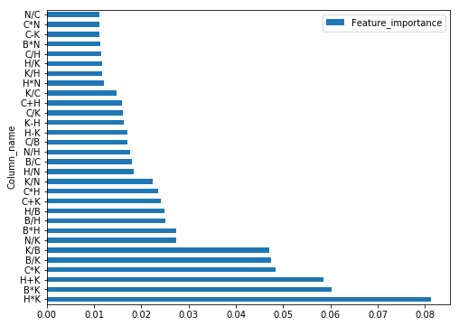
From the feature importances obtained we’ll use the top 15 interaction terms for further modelling.
feat_imp_intr = feat_imp.sort_values(by=['Feature_importance'],ascending=False).head(15)['Column_name'].values.tolist()
Final XGBOOST model with original and engineered features
##XGBOOST
from xgboost import XGBClassifier
xgb_model = XGBClassifier()
param_dist = {"max_depth": [5,10,30,50],
              "min_child_weight" : [1,3,6],
              "n_estimators": [200,500],
              "learning_rate": [0.05, 0.1,0.16],}
grid_search = GridSearchCV(xgb_model, param_grid=param_dist, cv = 3,
                                   verbose=10, n_jobs=-1)
grid_search.fit(train_enc[numerical+enc_freq_cols+enc_mean_cat+feat_interact],train_enc['P'])
Fitting 3 folds for each of 72 candidates, totalling 216 fits


[Parallel(n_jobs=-1)]: Using backend LokyBackend with 16 concurrent workers.
[Parallel(n_jobs=-1)]: Done   9 tasks      | elapsed:    3.6s
[Parallel(n_jobs=-1)]: Done  18 tasks      | elapsed:    4.4s
[Parallel(n_jobs=-1)]: Done  29 tasks      | elapsed:    5.3s
[Parallel(n_jobs=-1)]: Done  40 tasks      | elapsed:    5.8s
[Parallel(n_jobs=-1)]: Done  53 tasks      | elapsed:    6.8s
[Parallel(n_jobs=-1)]: Done  66 tasks      | elapsed:    7.7s
[Parallel(n_jobs=-1)]: Done  81 tasks      | elapsed:    8.4s
[Parallel(n_jobs=-1)]: Done  96 tasks      | elapsed:    9.2s
[Parallel(n_jobs=-1)]: Done 113 tasks      | elapsed:   10.1s
[Parallel(n_jobs=-1)]: Done 130 tasks      | elapsed:   11.0s
[Parallel(n_jobs=-1)]: Done 149 tasks      | elapsed:   11.9s
[Parallel(n_jobs=-1)]: Done 168 tasks      | elapsed:   12.8s
[Parallel(n_jobs=-1)]: Done 207 out of 216 | elapsed:   14.6s remaining:    0.6s
[Parallel(n_jobs=-1)]: Done 216 out of 216 | elapsed:   14.9s finished


GridSearchCV(cv=3, error_score='raise-deprecating',
       estimator=XGBClassifier(base_score=0.5, booster='gbtree', colsample_bylevel=1,
       colsample_bytree=1, gamma=0, learning_rate=0.1, max_delta_step=0,
       max_depth=3, min_child_weight=1, missing=None, n_estimators=100,
       n_jobs=1, nthread=None, objective='binary:logistic', random_state=0,
       reg_alpha=0, reg_lambda=1, scale_pos_weight=1, seed=None,
       silent=True, subsample=1),
       fit_params=None, iid='warn', n_jobs=-1,
       param_grid={'max_depth': [5, 10, 30, 50], 'min_child_weight': [1, 3, 6], 'n_estimators': [200, 500], 'learning_rate': [0.05, 0.1, 0.16]},
       pre_dispatch='2*n_jobs', refit=True, return_train_score='warn',
       scoring=None, verbose=10)
check_xgb = grid_search.best_estimator_
scores = cross_val_score(check_xgb,train_enc[numerical+enc_freq_cols+enc_mean_cat+feat_interact],train_enc['P'],cv=5,scoring='roc_auc')
scores.mean()
0.9397149548343927
As we can see,the interaction features definitely has improved the performance of our model.
grid_search.best_params_
{'learning_rate': 0.1,
 'max_depth': 5,
 'min_child_weight': 1,
 'n_estimators': 200}
final_xgb_params = {'learning_rate': 0.1,
 'max_depth': 5,
 'min_child_weight': 1,
 'n_estimators': 200}
xgb_final = XGBClassifier(**final_xgb_params)
xgb_final.fit(train_enc[numerical+enc_freq_cols+enc_mean_cat+feat_interact],train_enc['P'])
XGBClassifier(base_score=0.5, booster='gbtree', colsample_bylevel=1,
       colsample_bytree=1, gamma=0, learning_rate=0.1, max_delta_step=0,
       max_depth=5, min_child_weight=1, missing=None, n_estimators=200,
       n_jobs=1, nthread=None, objective='binary:logistic', random_state=0,
       reg_alpha=0, reg_lambda=1, scale_pos_weight=1, seed=None,
       silent=True, subsample=1)
final_preds = xgb_final.predict(test_enc[numerical+enc_freq_cols+enc_mean_cat+feat_interact])
#initial submission
submissions=pd.DataFrame(columns=['id', 'P'])
submissions['id']=test_df['id']
submissions['P']=final_preds
submissions.to_csv('mmtsub2.csv', index=False)
pred = pd.read_csv('mmtsub2.csv')
We can perform ensembling to improve predictions and we could tune the hyperparameters further as well to improve performance of model.