Housing Prices - Regression - Kaggle
Predict sales prices and practice feature engineering, RFs, and gradient boosting
Ask a home buyer to describe their dream house, and they probably won’t begin with the height of the basement ceiling or the proximity to an east-west railroad. But this playground competition’s dataset proves that much more influences price negotiations than the number of bedrooms or a white-picket fence.
With 79 explanatory variables describing (almost) every aspect of residential homes in Ames, Iowa, this competition challenges you to predict the final price of each home.
#main modules
import numpy as np
import pandas as pd
import matplotlib.pyplot as plt
%matplotlib inline
plt.rcParams['figure.figsize'] = (10.0, 8.0)
import seaborn as sns
from scipy import stats
from scipy.stats import norm
Load the csv data into dataframes
#read the data from csv files into dataframes
train_df = pd.read_csv('train.csv')
test_df = pd.read_csv('test.csv')
#print out no of rows and columns in Train and test data
print('Train data:-\n Columns: {}  Rows: {}'.format(train_df.shape[1],train_df.shape[0]))
print('Test data:-\n Columns: {}  Rows: {}'.format(test_df.shape[1],test_df.shape[0]))
Train data:-
 Columns: 81  Rows: 1460
Test data:-
 Columns: 80  Rows: 1459
train_df.head()
| Id | MSSubClass | MSZoning | LotFrontage | LotArea | Street | Alley | LotShape | LandContour | Utilities | ... | PoolArea | PoolQC | Fence | MiscFeature | MiscVal | MoSold | YrSold | SaleType | SaleCondition | SalePrice | |
|---|---|---|---|---|---|---|---|---|---|---|---|---|---|---|---|---|---|---|---|---|---|
| 0 | 1 | 60 | RL | 65.0 | 8450 | Pave | NaN | Reg | Lvl | AllPub | ... | 0 | NaN | NaN | NaN | 0 | 2 | 2008 | WD | Normal | 208500 |
| 1 | 2 | 20 | RL | 80.0 | 9600 | Pave | NaN | Reg | Lvl | AllPub | ... | 0 | NaN | NaN | NaN | 0 | 5 | 2007 | WD | Normal | 181500 |
| 2 | 3 | 60 | RL | 68.0 | 11250 | Pave | NaN | IR1 | Lvl | AllPub | ... | 0 | NaN | NaN | NaN | 0 | 9 | 2008 | WD | Normal | 223500 |
| 3 | 4 | 70 | RL | 60.0 | 9550 | Pave | NaN | IR1 | Lvl | AllPub | ... | 0 | NaN | NaN | NaN | 0 | 2 | 2006 | WD | Abnorml | 140000 |
| 4 | 5 | 60 | RL | 84.0 | 14260 | Pave | NaN | IR1 | Lvl | AllPub | ... | 0 | NaN | NaN | NaN | 0 | 12 | 2008 | WD | Normal | 250000 |
5 rows × 81 columns
test_df.head()
| Id | MSSubClass | MSZoning | LotFrontage | LotArea | Street | Alley | LotShape | LandContour | Utilities | ... | ScreenPorch | PoolArea | PoolQC | Fence | MiscFeature | MiscVal | MoSold | YrSold | SaleType | SaleCondition | |
|---|---|---|---|---|---|---|---|---|---|---|---|---|---|---|---|---|---|---|---|---|---|
| 0 | 1461 | 20 | RH | 80.0 | 11622 | Pave | NaN | Reg | Lvl | AllPub | ... | 120 | 0 | NaN | MnPrv | NaN | 0 | 6 | 2010 | WD | Normal |
| 1 | 1462 | 20 | RL | 81.0 | 14267 | Pave | NaN | IR1 | Lvl | AllPub | ... | 0 | 0 | NaN | NaN | Gar2 | 12500 | 6 | 2010 | WD | Normal |
| 2 | 1463 | 60 | RL | 74.0 | 13830 | Pave | NaN | IR1 | Lvl | AllPub | ... | 0 | 0 | NaN | MnPrv | NaN | 0 | 3 | 2010 | WD | Normal |
| 3 | 1464 | 60 | RL | 78.0 | 9978 | Pave | NaN | IR1 | Lvl | AllPub | ... | 0 | 0 | NaN | NaN | NaN | 0 | 6 | 2010 | WD | Normal |
| 4 | 1465 | 120 | RL | 43.0 | 5005 | Pave | NaN | IR1 | HLS | AllPub | ... | 144 | 0 | NaN | NaN | NaN | 0 | 1 | 2010 | WD | Normal |
5 rows × 80 columns
#combine both train and test data
#df=train_df.append(test_df,ignore_index=True)
df=pd.concat([train_df,test_df])
df.shape
(2919, 81)
Get feel of data
##only numeric columns
df.describe()
| 1stFlrSF | 2ndFlrSF | 3SsnPorch | BedroomAbvGr | BsmtFinSF1 | BsmtFinSF2 | BsmtFullBath | BsmtHalfBath | BsmtUnfSF | EnclosedPorch | ... | OverallQual | PoolArea | SalePrice | ScreenPorch | TotRmsAbvGrd | TotalBsmtSF | WoodDeckSF | YearBuilt | YearRemodAdd | YrSold | |
|---|---|---|---|---|---|---|---|---|---|---|---|---|---|---|---|---|---|---|---|---|---|
| count | 2919.000000 | 2919.000000 | 2919.000000 | 2919.000000 | 2918.000000 | 2918.000000 | 2917.000000 | 2917.000000 | 2918.000000 | 2919.000000 | ... | 2919.000000 | 2919.000000 | 1460.000000 | 2919.000000 | 2919.000000 | 2918.000000 | 2919.000000 | 2919.000000 | 2919.000000 | 2919.000000 |
| mean | 1159.581706 | 336.483727 | 2.602261 | 2.860226 | 441.423235 | 49.582248 | 0.429894 | 0.061364 | 560.772104 | 23.098321 | ... | 6.089072 | 2.251799 | 180921.195890 | 16.062350 | 6.451524 | 1051.777587 | 93.709832 | 1971.312778 | 1984.264474 | 2007.792737 |
| std | 392.362079 | 428.701456 | 25.188169 | 0.822693 | 455.610826 | 169.205611 | 0.524736 | 0.245687 | 439.543659 | 64.244246 | ... | 1.409947 | 35.663946 | 79442.502883 | 56.184365 | 1.569379 | 440.766258 | 126.526589 | 30.291442 | 20.894344 | 1.314964 |
| min | 334.000000 | 0.000000 | 0.000000 | 0.000000 | 0.000000 | 0.000000 | 0.000000 | 0.000000 | 0.000000 | 0.000000 | ... | 1.000000 | 0.000000 | 34900.000000 | 0.000000 | 2.000000 | 0.000000 | 0.000000 | 1872.000000 | 1950.000000 | 2006.000000 |
| 25% | 876.000000 | 0.000000 | 0.000000 | 2.000000 | 0.000000 | 0.000000 | 0.000000 | 0.000000 | 220.000000 | 0.000000 | ... | 5.000000 | 0.000000 | 129975.000000 | 0.000000 | 5.000000 | 793.000000 | 0.000000 | 1953.500000 | 1965.000000 | 2007.000000 |
| 50% | 1082.000000 | 0.000000 | 0.000000 | 3.000000 | 368.500000 | 0.000000 | 0.000000 | 0.000000 | 467.000000 | 0.000000 | ... | 6.000000 | 0.000000 | 163000.000000 | 0.000000 | 6.000000 | 989.500000 | 0.000000 | 1973.000000 | 1993.000000 | 2008.000000 |
| 75% | 1387.500000 | 704.000000 | 0.000000 | 3.000000 | 733.000000 | 0.000000 | 1.000000 | 0.000000 | 805.500000 | 0.000000 | ... | 7.000000 | 0.000000 | 214000.000000 | 0.000000 | 7.000000 | 1302.000000 | 168.000000 | 2001.000000 | 2004.000000 | 2009.000000 |
| max | 5095.000000 | 2065.000000 | 508.000000 | 8.000000 | 5644.000000 | 1526.000000 | 3.000000 | 2.000000 | 2336.000000 | 1012.000000 | ... | 10.000000 | 800.000000 | 755000.000000 | 576.000000 | 15.000000 | 6110.000000 | 1424.000000 | 2010.000000 | 2010.000000 | 2010.000000 |
8 rows × 38 columns
#train_df.info()
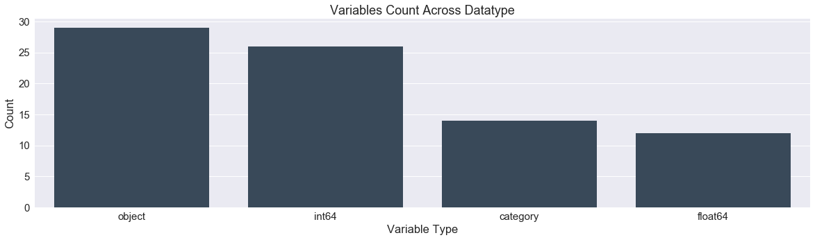
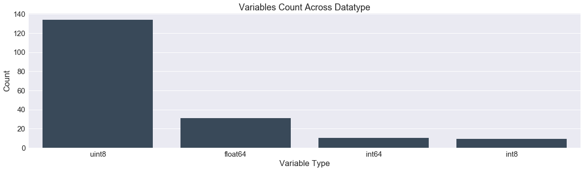
def variable_dtype_plot(df):
'''bar plot indicating the count of data types
present in the dataframe'''
df_dtype = pd.DataFrame(df.dtypes.value_counts()).reset_index().rename(columns={"index":"datatype",0:"count"})
fig,ax = plt.subplots()
fig.set_size_inches(20,5)
sns.barplot(data=df_dtype,x="datatype",y="count",ax=ax,color="#34495e")
ax.set(xlabel='Variable Type', ylabel='Count',title="Variables Count Across Datatype")
plt.show()
variable_dtype_plot(df)

#check no of each column types
df.dtypes.value_counts()
object     43
int64      26
float64    12
dtype: int64
#get numerical and categorical columns of dataframe into lists.
categorical = list(df.columns[df.dtypes=="object"])
numerical = list(df.columns[df.dtypes!="object"])
#use describe method on the categorical columns
df[categorical].describe()
| Alley | BldgType | BsmtCond | BsmtExposure | BsmtFinType1 | BsmtFinType2 | BsmtQual | CentralAir | Condition1 | Condition2 | ... | MiscFeature | Neighborhood | PavedDrive | PoolQC | RoofMatl | RoofStyle | SaleCondition | SaleType | Street | Utilities | |
|---|---|---|---|---|---|---|---|---|---|---|---|---|---|---|---|---|---|---|---|---|---|
| count | 198 | 2919 | 2837 | 2837 | 2840 | 2839 | 2838 | 2919 | 2919 | 2919 | ... | 105 | 2919 | 2919 | 10 | 2919 | 2919 | 2919 | 2918 | 2919 | 2917 |
| unique | 2 | 5 | 4 | 4 | 6 | 6 | 4 | 2 | 9 | 8 | ... | 4 | 25 | 3 | 3 | 8 | 6 | 6 | 9 | 2 | 2 |
| top | Grvl | 1Fam | TA | No | Unf | Unf | TA | Y | Norm | Norm | ... | Shed | NAmes | Y | Gd | CompShg | Gable | Normal | WD | Pave | AllPub |
| freq | 120 | 2425 | 2606 | 1904 | 851 | 2493 | 1283 | 2723 | 2511 | 2889 | ... | 95 | 443 | 2641 | 4 | 2876 | 2310 | 2402 | 2525 | 2907 | 2916 |
4 rows × 43 columns
Exploratory Data Analysis
analytically exploring data in order to provide some insights for subsequent processing and modeling.
Usually we would load the data using Pandas and make some visualizations to understand the data.
Inspect the distribution of target variable. Depending on what scoring metric is used, an imbalanced distribution of target variable might harm the model’s performance.
For numerical variables, use box plot and scatter plot to inspect their distributions and check for outliers.
For classification tasks, plot the data with points colored according to their labels. This can help with feature engineering.
Make pairwise distribution plots and examine their correlations.
https://www.kaggle.com/benhamner/d/uciml/iris/python-data-visualizations
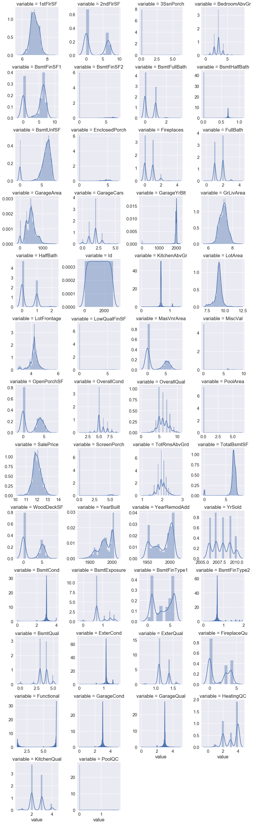
#univariate analysis
##plotting histograms to find distribution of continuous variables in dataset
#num = [f for f in df.columns if df.dtypes[f] != 'object']
numdf=pd.melt(train_df,value_vars=numerical)
numgrid=sns.FacetGrid(numdf,col='variable',col_wrap=5,sharex=False,sharey=False)
numgrid=numgrid.map(sns.distplot,'value')
numgrid
<seaborn.axisgrid.FacetGrid at 0x210818eb080>

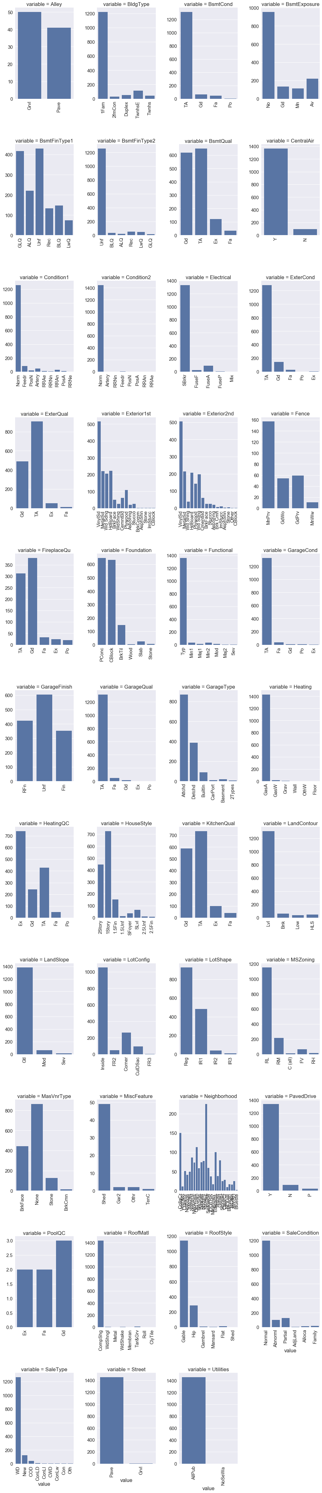
##count plot of categorical attributes
#col = [f for f in train_df.columns if train_df.dtypes[f] == 'object']
coldf=pd.melt(train_df,value_vars=categorical)
colgrid=sns.FacetGrid(coldf,col='variable',col_wrap=4,size=6,aspect=.6,sharex=False,sharey=False)
plt.xticks(rotation=90)
colgrid = colgrid.map(sns.countplot,'value')
plt.tight_layout()
plt.subplots_adjust(hspace=0.5, wspace=0.4)


###rotating x axis labels to prevent overlapping
for ax in colgrid.axes:
    for label in ax.get_xticklabels():
        label.set_rotation(90)
colgrid
<seaborn.axisgrid.FacetGrid at 0x210859a5320>
def boxplot(x,y,**kwargs):
            sns.boxplot(x=x,y=y)
            x = plt.xticks(rotation=90)

#cat = [f for f in train_df.columns if train_df.dtypes[f] == 'object']

p = pd.melt(train_df, id_vars='SalePrice', value_vars=categorical)
g = sns.FacetGrid (p, col='variable', col_wrap=2, sharex=False, sharey=False, size=5)
g = g.map(boxplot, 'value','SalePrice')
g
<seaborn.axisgrid.FacetGrid at 0x21083ae2898>

Data Preprocessing
Note that we combined the data from our training and test sets into a single dataframe here (called df), dropping our target variable (SalePrice). These numbers thus represent the total number of missing values across the full dataset. Since the total number of entries in our train and test sets is 2919, we can see that for some features nearly all entries are missing, while for others it is just one or two. How we proceed to treat these missing values depends very much on the reasons the data is missing, the problem and the type of model we want to use.
Checking for null values ,missing data
#sns.pairplot(train_df[['LotFrontage','LotArea']],diag_kind="hist")
#check the columns which are having any null values
#train_df.columns[train_df.isnull().any()]
print('    >>>>>Numerical variables having nulls and its counts<<<<<<<<')
num_nulls = df[numerical].isnull().sum()[df[numerical].isnull().sum()>0].sort_values(ascending=False)
num_nulls
    >>>>>Numerical variables having nulls and its counts<<<<<<<<


SalePrice       1459
LotFrontage      486
GarageYrBlt      159
MasVnrArea        23
BsmtHalfBath       2
BsmtFullBath       2
TotalBsmtSF        1
GarageCars         1
GarageArea         1
BsmtUnfSF          1
BsmtFinSF2         1
BsmtFinSF1         1
dtype: int64
print('      >>>>>Categorical variables having nulls and its counts<<<<<<<<')
col_nulls = df[categorical].isnull().sum()[df[categorical].isnull().sum()>0].sort_values(ascending=False)
col_nulls
      >>>>>Categorical variables having nulls and its counts<<<<<<<<


PoolQC          2909
MiscFeature     2814
Alley           2721
Fence           2348
FireplaceQu     1420
GarageQual       159
GarageFinish     159
GarageCond       159
GarageType       157
BsmtCond          82
BsmtExposure      82
BsmtQual          81
BsmtFinType2      80
BsmtFinType1      79
MasVnrType        24
MSZoning           4
Utilities          2
Functional         2
Electrical         1
Exterior1st        1
Exterior2nd        1
SaleType           1
KitchenQual        1
dtype: int64
Treating Null values
We could either delete,impute or leave null values based on algorithms used.
On checking the distribution of ‘LotFrontage’ variable in below univariate analysis hist plot,we can see that data is skewed left,therefore we use the median value to impute missing value here
df['LotFrontage'].fillna(df['LotFrontage'].median(),inplace=True)
We will fill ‘GarageYrBlt’ variable null values with zero for now as it indicates no garage built.
If we look at the data description,missing values indicates meaningful data and we need to fill with 0 instead.
This might be used to create new feature in feature engineering.
df['GarageYrBlt'].fillna(0, inplace=True)
df.MasVnrArea.fillna(0, inplace=True)
df.BsmtHalfBath.fillna(0, inplace=True)
df.BsmtFullBath.fillna(0, inplace=True)
df.GarageArea.fillna(0, inplace=True)
df.GarageCars.fillna(0, inplace=True)
df.TotalBsmtSF.fillna(0, inplace=True)
df.BsmtUnfSF.fillna(0, inplace=True)
df.BsmtFinSF2.fillna(0, inplace=True)
df.BsmtFinSF1.fillna(0, inplace=True)
Now we have imputed missing values in numerical variables.Lets check the categorical variables null values.In case of PoolQC we can drop this whole column due to large null values and infering less dependancy with target variable.For now we will impute ‘NA’ as pool area for these is also 0.
df.loc[df['PoolQC'].isnull()==True,['PoolArea','PoolQC']].describe()
df.PoolQC.fillna('NA', inplace=True)
df.MiscFeature.fillna('NA', inplace=True)
df.Alley.fillna('NA', inplace=True)
df.Fence.fillna('NA', inplace=True)
df.FireplaceQu.fillna('NA', inplace=True)
df.GarageCond.fillna('NA', inplace=True)
df.GarageQual.fillna('NA', inplace=True)
df.GarageFinish.fillna('NA', inplace=True)
df.GarageType.fillna('NA', inplace=True)
df.BsmtExposure.fillna('NA', inplace=True)
df.BsmtCond.fillna('NA', inplace=True)
df.BsmtQual.fillna('NA', inplace=True)
df.BsmtFinType2.fillna('NA', inplace=True)
df.BsmtFinType1.fillna('NA', inplace=True)
df.MasVnrType.fillna('None', inplace=True)
df.Exterior2nd.fillna('None', inplace=True)
We could predict these values based on other similar variable in our data using knn algorithm,for example MSZoning variable.for now we can impute or drop rows having nulls of this variable.
#df.dropna(subset =['MSZoning'],inplace=True)
df.Functional.fillna(df.Functional.mode()[0], inplace=True)
df.Utilities.fillna(df.Utilities.mode()[0], inplace=True)
df.Exterior1st.fillna(df.Exterior1st.mode()[0], inplace=True)
df.SaleType.fillna(df.SaleType.mode()[0], inplace=True)
df.KitchenQual.fillna(df.KitchenQual.mode()[0], inplace=True)
df.Electrical.fillna(df.Electrical.mode()[0], inplace=True)
For now,we have handled null values,we can always comeback and use different imputation strategies
Treating Outliers
@@@@@@@@@To be performed …left out as we would try tree based models which would be less prone to outliers@@@@@@@@@
Categorical variables encoding
http://pbpython.com/categorical-encoding.html Use either numeric encoding or one-hot encoding. As a guide, you’ll want to use one-hot encodind when there’s no inherent order to your category, and numeric otherwise.
From the variable with object dtype we can infer that few are nominal and ordinal,we select these and perform encoding on these.
##selecting few cat features to be encoded.
cols_tobe_encoded= ['Alley','BsmtCond','BsmtExposure', 'BsmtFinType1','BsmtFinType2','BsmtQual', 'ExterCond','ExterQual' ,'FireplaceQu',
                    'Functional','GarageCond', 'GarageQual', 'HeatingQC','KitchenQual','LandSlope', 'PavedDrive', 'PoolQC', 'Street', 'Utilities' ]
df[cols_tobe_encoded].describe()
| Alley | BsmtCond | BsmtExposure | BsmtFinType1 | BsmtFinType2 | BsmtQual | ExterCond | ExterQual | FireplaceQu | Functional | GarageCond | GarageQual | HeatingQC | KitchenQual | LandSlope | PavedDrive | PoolQC | Street | Utilities | |
|---|---|---|---|---|---|---|---|---|---|---|---|---|---|---|---|---|---|---|---|
| count | 2919 | 2919 | 2919 | 2919 | 2919 | 2919 | 2919 | 2919 | 2919 | 2919 | 2919 | 2919 | 2919 | 2919 | 2919 | 2919 | 2919 | 2919 | 2919 |
| unique | 3 | 5 | 5 | 7 | 7 | 5 | 5 | 4 | 6 | 7 | 6 | 6 | 5 | 4 | 3 | 3 | 4 | 2 | 2 |
| top | NA | TA | No | Unf | Unf | TA | TA | TA | NA | Typ | TA | TA | Ex | TA | Gtl | Y | NA | Pave | AllPub |
| freq | 2721 | 2606 | 1904 | 851 | 2493 | 1283 | 2538 | 1798 | 1420 | 2719 | 2654 | 2604 | 1493 | 1493 | 2778 | 2641 | 2909 | 2907 | 2918 |
##categorical features having inherent ordering
ordinal_cat_cols= ['BsmtCond','BsmtExposure', 'BsmtFinType1','BsmtFinType2','BsmtQual', 'ExterCond','ExterQual' ,'FireplaceQu',
                    'Functional','GarageCond', 'GarageQual', 'HeatingQC','KitchenQual', 'PoolQC',]
##categorical features which are nominal
nominal_cat_cols= [i for i in cols_tobe_encoded if i not in ordinal_cat_cols]
print(nominal_cat_cols)
['Alley', 'LandSlope', 'PavedDrive', 'Street', 'Utilities']
[i for i in categorical if i not in cols_tobe_encoded]
['BldgType',
 'CentralAir',
 'Condition1',
 'Condition2',
 'Electrical',
 'Exterior1st',
 'Exterior2nd',
 'Fence',
 'Foundation',
 'GarageFinish',
 'GarageType',
 'Heating',
 'HouseStyle',
 'LandContour',
 'LotConfig',
 'LotShape',
 'MSZoning',
 'MasVnrType',
 'MiscFeature',
 'Neighborhood',
 'RoofMatl',
 'RoofStyle',
 'SaleCondition',
 'SaleType']
dummy variables tend to increase the multicollinearity in our dataset,therefore it is important to check VIF later and remove high multicollinear variable http://www.algosome.com/articles/dummy-variable-trap-regression.html
df['BsmtCond']=df['BsmtCond'].astype('category',
                             categories=['NA','Po','Fa','TA','Gd','Ex'],
                             ordered=True)
#######
df['ExterQual']=df['ExterQual'].astype('category',
                             categories=['Po','Fa','TA','Gd','Ex'],
                             ordered=True)
#######
df['KitchenQual']=df['KitchenQual'].astype('category',
                             categories=['Po','Fa','TA','Gd','Ex'],
                             ordered=True)

#######
df['PoolQC']=df['PoolQC'].astype('category',
                             categories=['NA','Po','Fa','TA','Gd','Ex'],
                             ordered=True)
df['BsmtExposure']=df['BsmtExposure'].astype('category',
                             categories=['NA','No','Mn','Av','Gd'],
                             ordered=True)

df['BsmtFinType1']=df['BsmtFinType1'].astype('category',
                             categories=['NA','Unf', 'LwQ', 'Rec', 'BLQ', 'ALQ', 'GLQ'],
                             ordered=True)

df['BsmtFinType2']=df['BsmtFinType2'].astype('category',
                             categories=['NA','Unf', 'LwQ', 'Rec', 'BLQ', 'ALQ', 'GLQ'],
                             ordered=True)

df['BsmtQual']=df['BsmtQual'].astype('category',
                             categories=['NA','Po','Fa','TA','Gd','Ex'],
                             ordered=True)
df['ExterCond']=df['ExterCond'].astype('category',
                             categories=['Po','Fa','TA','Gd','Ex'],
                                       ordered=True)


df['FireplaceQu']=df['FireplaceQu'].astype('category',
                             categories=['NA','Po','Fa','TA','Gd','Ex'],
                             ordered=True)
df['Functional']=df['Functional'].astype('category',
                             categories=['Sal', 'Sev', 'Maj2', 'Maj1', 'Mod', 'Min2', 'Min1', 'Typ'],
                             ordered=True)

df['GarageQual']=df['GarageQual'].astype('category',
                             categories=['NA','Po','Fa','TA','Gd','Ex'],
                             ordered=True)

df['GarageCond']=df['GarageCond'].astype('category',
                             categories=['NA','Po','Fa','TA','Gd','Ex'],
                             ordered=True)

df['HeatingQC']=df['HeatingQC'].astype('category',
                             categories=['Po','Fa','TA','Gd','Ex'],
                             ordered=True)
variable_dtype_plot(df)
ordinal_cat_cols= ['BsmtCond','BsmtExposure', 'BsmtFinType1','BsmtFinType2','BsmtQual', 'ExterCond','ExterQual' ,'FireplaceQu',
                    'Functional','GarageCond', 'GarageQual', 'HeatingQC','KitchenQual', 'PoolQC',]

for col in ordinal_cat_cols:
    df[col] = df[col].cat.codes
##update list of numerical features and categorical features
numerical = numerical + ordinal_cat_cols

for col in ordinal_cat_cols:
    categorical.remove(col)
Now we have marked the ordinal columns which are encoded as nos to be numerical features and removed them from categorical features list.
Now the columns remaining in categorical features list would need to be one-hot encoded as there is no inherent ordering in the column values.
df[categorical].describe().T
| count | unique | top | freq | |
|---|---|---|---|---|
| Alley | 2919 | 3 | NA | 2721 |
| BldgType | 2919 | 5 | 1Fam | 2425 |
| CentralAir | 2919 | 2 | Y | 2723 |
| Condition1 | 2919 | 9 | Norm | 2511 |
| Condition2 | 2919 | 8 | Norm | 2889 |
| Electrical | 2919 | 5 | SBrkr | 2672 |
| Exterior1st | 2919 | 15 | VinylSd | 1026 |
| Exterior2nd | 2919 | 17 | VinylSd | 1014 |
| Fence | 2919 | 5 | NA | 2348 |
| Foundation | 2919 | 6 | PConc | 1308 |
| GarageFinish | 2919 | 4 | Unf | 1230 |
| GarageType | 2919 | 7 | Attchd | 1723 |
| Heating | 2919 | 6 | GasA | 2874 |
| HouseStyle | 2919 | 8 | 1Story | 1471 |
| LandContour | 2919 | 4 | Lvl | 2622 |
| LandSlope | 2919 | 3 | Gtl | 2778 |
| LotConfig | 2919 | 5 | Inside | 2133 |
| LotShape | 2919 | 4 | Reg | 1859 |
| MSZoning | 2915 | 5 | RL | 2265 |
| MasVnrType | 2919 | 4 | None | 1766 |
| MiscFeature | 2919 | 5 | NA | 2814 |
| Neighborhood | 2919 | 25 | NAmes | 443 |
| PavedDrive | 2919 | 3 | Y | 2641 |
| RoofMatl | 2919 | 8 | CompShg | 2876 |
| RoofStyle | 2919 | 6 | Gable | 2310 |
| SaleCondition | 2919 | 6 | Normal | 2402 |
| SaleType | 2919 | 9 | WD | 2526 |
| Street | 2919 | 2 | Pave | 2907 |
| Utilities | 2919 | 2 | AllPub | 2918 |
##these variables tend to have no inherent ordering in their values
#df = pd.get_dummies(df,columns=['Alley','LandSlope','PavedDrive','Street','Utilities'])
There are still a few non-numerical data in our dataframe which needs to be encoded using one of the techniques.
##MSSubClass is a category feature and needs to be encoded as categories.
df.replace({'MSSubClass':{20:'class1', 30:'class2', 40:'class3', 45:'class4',
                                   50:'class5', 60:'class6', 70:'class7', 75:'class8',
                                   80:'class9', 85:'class10', 90:'class11', 120:'class12',
                                   150:'class13', 160:'class14', 180:'class15', 190:'class16'}},inplace=True)

df['MSSubClass'] = df['MSSubClass'].astype('category')
##update categorical features

categorical.append('MSSubClass')
numerical.remove('MSSubClass')
df[categorical].describe()
| Alley | BldgType | CentralAir | Condition1 | Condition2 | Electrical | Exterior1st | Exterior2nd | Fence | Foundation | ... | MiscFeature | Neighborhood | PavedDrive | RoofMatl | RoofStyle | SaleCondition | SaleType | Street | Utilities | MSSubClass | |
|---|---|---|---|---|---|---|---|---|---|---|---|---|---|---|---|---|---|---|---|---|---|
| count | 2919 | 2919 | 2919 | 2919 | 2919 | 2919 | 2919 | 2919 | 2919 | 2919 | ... | 2919 | 2919 | 2919 | 2919 | 2919 | 2919 | 2919 | 2919 | 2919 | 2919 |
| unique | 3 | 5 | 2 | 9 | 8 | 5 | 15 | 17 | 5 | 6 | ... | 5 | 25 | 3 | 8 | 6 | 6 | 9 | 2 | 2 | 16 |
| top | NA | 1Fam | Y | Norm | Norm | SBrkr | VinylSd | VinylSd | NA | PConc | ... | NA | NAmes | Y | CompShg | Gable | Normal | WD | Pave | AllPub | class1 |
| freq | 2721 | 2425 | 2723 | 2511 | 2889 | 2672 | 1026 | 1014 | 2348 | 1308 | ... | 2814 | 443 | 2641 | 2876 | 2310 | 2402 | 2526 | 2907 | 2918 | 1079 |
4 rows × 30 columns
As we can see,there are many categories in Neigborhood attribute(25),we will analyze this attribute and combine levels of the neighborhood variable into fewer levels.
We plot below the median of saleprice wrt to each neighborhood type and it gives us an idea to combine levels with similar height into a single level.
train_df.groupby('Neighborhood')['SalePrice'].agg({'median':np.median}).sort_values(by='median').plot(kind='bar')
C:\Users\Nithin\Anaconda3\lib\site-packages\ipykernel_launcher.py:1: FutureWarning: using a dict on a Series for aggregation
is deprecated and will be removed in a future version
  """Entry point for launching an IPython kernel.


<matplotlib.axes._subplots.AxesSubplot at 0x2109188f860>
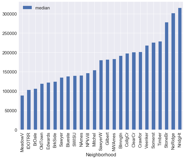
neighborhood_map = {"MeadowV" : 0, "IDOTRR" : 1, "BrDale" : 1, "OldTown" : 1, "Edwards" : 1,
                    "BrkSide" : 1,"Sawyer" : 1, "Blueste" : 1, "SWISU" : 2, "NAmes" : 2,
                    "NPkVill" : 2, "Mitchel" : 2, "SawyerW" : 2, "Gilbert" : 2, "NWAmes" : 2,
                    "Blmngtn" : 2, "CollgCr" : 2, "ClearCr" : 3, "Crawfor" : 3, "Veenker" : 3,
                    "Somerst" : 3, "Timber" : 3, "StoneBr" : 4, "NoRidge" : 4, "NridgHt" : 4}

df.replace({'Neighborhood':neighborhood_map},inplace=True)

df['Neighborhood'] = df['Neighborhood'].astype('category')
train_df.groupby('Exterior1st')['SalePrice'].agg({'median':np.median}).sort_values(by='median').plot(kind='bar')
C:\Users\Nithin\Anaconda3\lib\site-packages\ipykernel_launcher.py:1: FutureWarning: using a dict on a Series for aggregation
is deprecated and will be removed in a future version
  """Entry point for launching an IPython kernel.


<matplotlib.axes._subplots.AxesSubplot at 0x210916a9a58>
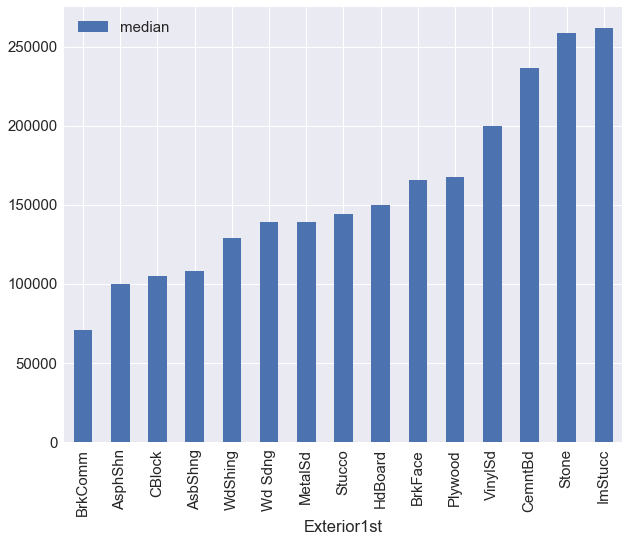
exterior1st_map = {"BrkComm":1,"AsphShn":1,"CBlock":1,"AsbShng":1,"WdShing":2,
                  "Wd Sdng":2,"MetalSd":2,"Stucco":2,"HdBoard":2,"BrkFace":3,"Plywood":3,
                  "VinylSd":4,"CemntBd":4,"Stone":4,"ImStucc":4,}

df.replace({'Exterior1st':exterior1st_map},inplace=True)

df['Exterior1st'] = df['Exterior1st'].astype('category')
train_df.groupby('Exterior2nd')['SalePrice'].agg({'median':np.median}).sort_values(by='median').plot(kind='bar')
C:\Users\Nithin\Anaconda3\lib\site-packages\ipykernel_launcher.py:1: FutureWarning: using a dict on a Series for aggregation
is deprecated and will be removed in a future version
  """Entry point for launching an IPython kernel.


<matplotlib.axes._subplots.AxesSubplot at 0x210917dd0f0>
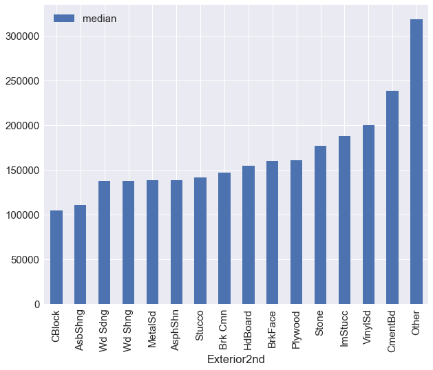
exterior2nd_map = {'VinylSd':3, 'MetalSd':2, 'Wd Shng':2, 'HdBoard':2, 'Plywood':2, 'Wd Sdng':2,
       'CmentBd':4, 'BrkFace':2, 'Stucco':2, 'AsbShng':1, 'Brk Cmn':2, 'ImStucc':3,
       'AsphShn':2, 'Stone':2, 'Other':4, 'CBlock':1, 'None':0}

df.replace({'Exterior2nd':exterior2nd_map},inplace=True)

df['Exterior2nd'] = df['Exterior2nd'].astype('category')
df[categorical].describe().T
| count | unique | top | freq | |
|---|---|---|---|---|
| Alley | 2919 | 3 | NA | 2721 |
| BldgType | 2919 | 5 | 1Fam | 2425 |
| CentralAir | 2919 | 2 | Y | 2723 |
| Condition1 | 2919 | 9 | Norm | 2511 |
| Condition2 | 2919 | 8 | Norm | 2889 |
| Electrical | 2919 | 5 | SBrkr | 2672 |
| Exterior1st | 2919 | 4 | 2 | 1402 |
| Exterior2nd | 2919 | 5 | 2 | 1721 |
| Fence | 2919 | 5 | NA | 2348 |
| Foundation | 2919 | 6 | PConc | 1308 |
| GarageFinish | 2919 | 4 | Unf | 1230 |
| GarageType | 2919 | 7 | Attchd | 1723 |
| Heating | 2919 | 6 | GasA | 2874 |
| HouseStyle | 2919 | 8 | 1Story | 1471 |
| LandContour | 2919 | 4 | Lvl | 2622 |
| LandSlope | 2919 | 3 | Gtl | 2778 |
| LotConfig | 2919 | 5 | Inside | 2133 |
| LotShape | 2919 | 4 | Reg | 1859 |
| MSZoning | 2915 | 5 | RL | 2265 |
| MasVnrType | 2919 | 4 | None | 1766 |
| MiscFeature | 2919 | 5 | NA | 2814 |
| Neighborhood | 2919 | 5 | 2 | 1344 |
| PavedDrive | 2919 | 3 | Y | 2641 |
| RoofMatl | 2919 | 8 | CompShg | 2876 |
| RoofStyle | 2919 | 6 | Gable | 2310 |
| SaleCondition | 2919 | 6 | Normal | 2402 |
| SaleType | 2919 | 9 | WD | 2526 |
| Street | 2919 | 2 | Pave | 2907 |
| Utilities | 2919 | 2 | AllPub | 2918 |
| MSSubClass | 2919 | 16 | class1 | 1079 |
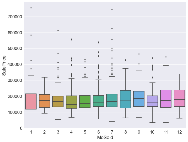
###we will drop the month sold as it does not impact the saleprice
df.drop('MoSold',axis=1,inplace=True)
#numerical.remove('MoSold')
numerical.remove('MoSold')
sns.boxplot(x='MoSold',y='SalePrice', data=train_df)
<matplotlib.axes._subplots.AxesSubplot at 0x21092f44ac8>
#df = pd.get_dummies(df,columns=categorical,drop_first=True)
###now we have 213 columns due to one-hot encoding
df.shape
(2919, 80)
###now we plot the distribution of numerical variables in our dataset
#num = [f for f in df.columns if df.dtypes[f] != 'object']
numdf=pd.melt(df,value_vars=numerical)
numgrid=sns.FacetGrid(numdf,col='variable',col_wrap=4,sharex=False,sharey=False)
numgrid=numgrid.map(sns.distplot,'value')
numgrid
<seaborn.axisgrid.FacetGrid at 0x210935ac588>
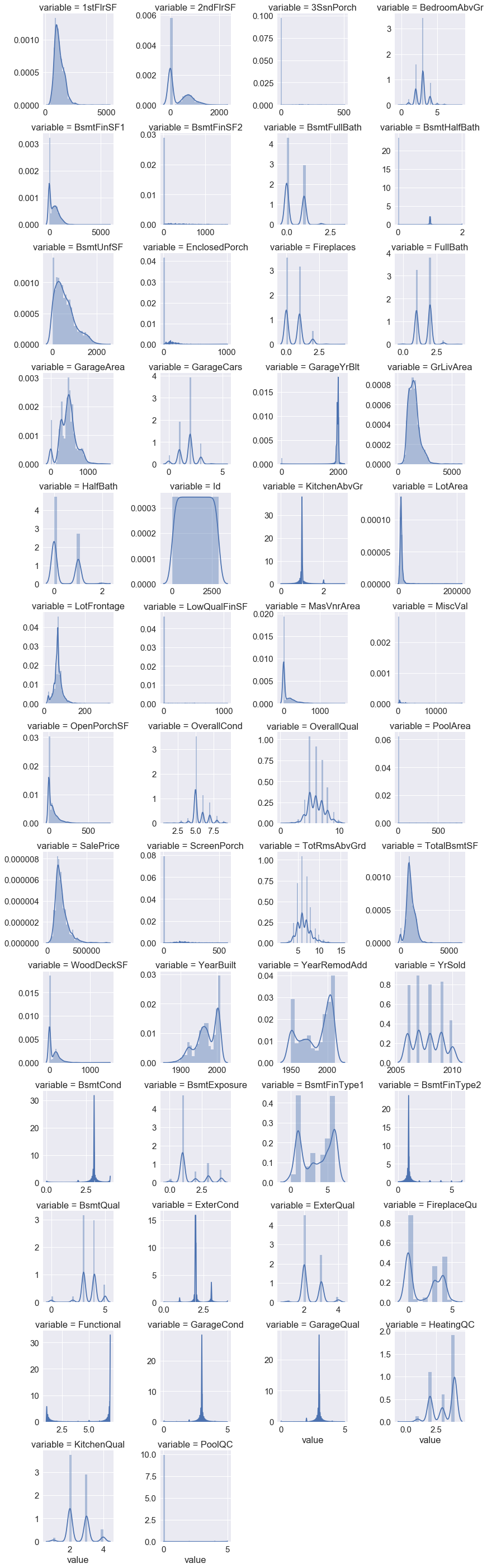
We see that the target variable SalePrice has a right-skewed distribution. We’ll need to log transform this variable so that it becomes normally distributed. A normally distributed (or close to normal) target variable helps in better modeling the relationship between target and independent variables. In addition, linear algorithms assume constant variance in the error term. Alternatively, we can also confirm this skewed behavior using the skewness metric. ,final result is evaluated using the Root-Mean-Squared-Error (RMSE) between the logarithm of the predicted value and the logarithm of the observed sales price,therefore it would be better to log-transform this variable
print ("The skewness of SalePrice is {}".format(df['SalePrice'].skew()))
The skewness of SalePrice is 1.8828757597682129
target = np.log(df['SalePrice'].dropna())
print ('Skewness is', target.skew())
sns.distplot(target)
Skewness is 0.121335062205


<matplotlib.axes._subplots.AxesSubplot at 0x21099fb4240>
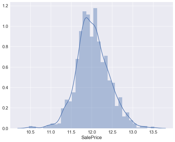
df['SalePrice'] = np.log(df['SalePrice'])
#df['SalePrice']
#numdf1 = pd.melt(train_df, id_vars=['SalePrice'],value_vars=numerical)
#numgrid1 = sns.FacetGrid(numdf1, col="variable",  col_wrap=4 , size=3.0,aspect=1.2,sharex=False, sharey=False)
#numgrid1.map(plt.scatter, "value",'SalePrice',s=1.5)
#numgrid1
from scipy.stats import skew
skewed = df[numerical].apply(lambda x: skew(x.dropna().astype(float)))
skewed = skewed[skewed>0.75].index
skewed
Index(['1stFlrSF', '2ndFlrSF', '3SsnPorch', 'BsmtFinSF1', 'BsmtFinSF2',
       'BsmtHalfBath', 'BsmtUnfSF', 'EnclosedPorch', 'GrLivArea',
       'KitchenAbvGr', 'LotArea', 'LotFrontage', 'LowQualFinSF', 'MasVnrArea',
       'MiscVal', 'OpenPorchSF', 'PoolArea', 'ScreenPorch', 'TotRmsAbvGrd',
       'TotalBsmtSF', 'WoodDeckSF', 'BsmtExposure', 'BsmtFinType2',
       'ExterCond', 'ExterQual', 'PoolQC'],
      dtype='object')
df[skewed]=np.log1p(df[skewed])
##we will plot the distributions again to check skewness
numdf=pd.melt(df,value_vars=numerical)
numgrid=sns.FacetGrid(numdf,col='variable',col_wrap=4,sharex=False,sharey=False)
numgrid=numgrid.map(sns.distplot,'value')
numgrid
<seaborn.axisgrid.FacetGrid at 0x21097addf98>
As we have already encoded ordinal categorical variables we are left with encoding the nominal categorical variables using one-hot encoding
df = pd.get_dummies(df,columns=categorical,drop_first=True)
df.shape
(2919, 184)
Now we have numerically encoded all our features as seen below in the plot of dtypes.We can now split the train and test data.
variable_dtype_plot(df)
X_train  = df[:1460].drop(['SalePrice','Id'], axis=1)
y_train  = df[:1460]['SalePrice']
X_test  = df[1460:].drop(['SalePrice','Id'], axis=1)
Now, we’ll standardize the numeric features.(those which are not dummy variables).Ensure to fit using train data and transform both train and test data
numerical.remove('SalePrice')
numerical.remove('Id')
from sklearn.preprocessing import StandardScaler
scaler = StandardScaler()
scaler.fit(X_train[numerical])
X_train[numerical]= scaler.transform(X_train[numerical])
X_test[numerical]= scaler.transform(X_test[numerical])
X_train.shape,y_train.shape,X_test.shape
((1460, 182), (1460,), (1459, 182))
Feature Selection
Decision trees are by nature immune to multi-collinearity. For example, if you have 2 features which are 99% correlated, when deciding upon a split the tree will choose only one of them. Other models such as Logistic regression would use both the features.
Since boosted trees use individual decision trees, they also are unaffected by multi-collinearity. However, its a good practice to remove any redundant features from any dataset used for training, irrespective of the model’s algorithm. In your case since you’re deriving new features, you could use this approach, evaluate each feature’s importance and retain only the best features for your final model.
Now there are 221 features due to a large amount of the dummy variable. Overfitting can easily occur when there are redundant features. Therefore I use XGBoost regressor to generate the rank of “feature importance”
import xgboost as xgb
from sklearn.model_selection import GridSearchCV
Parameters max_depth and min_child_weight Those parameters add constraints on the architecture of the trees.
i)max_depth is the maximum number of nodes allowed from the root to the farthest leaf of a tree. Deeper trees can model more complex relationships by adding more nodes, but as we go deeper, splits become less relevant and are sometimes only due to noise, causing the model to overfit.
ii)min_child_weight is the minimum weight (or number of samples if all samples have a weight of 1) required in order to create a new node in the tree. A smaller min_child_weight allows the algorithm to create children that correspond to fewer samples, thus allowing for more complex trees, but again, more likely to overfit. Thus, those parameters can be used to control the complexity of the trees.
It is important to tune them together in order to find a good trade-off between model bias and variance
param_grid = {'max_depth': [3,5,7], 'min_child_weight': [1,3,5]}
xgb_param = {'learning_rate': 0.1, 'n_estimators': 1000, 'seed':0, 'subsample': 0.8, 'colsample_bytree': 0.8,
             'objective': 'reg:linear'}
xgb_reg = xgb.XGBRegressor(**xgb_param)
optimize_xgb = GridSearchCV(estimator=xgb_reg,param_grid=param_grid,scoring='neg_mean_squared_error',cv = 5, n_jobs = -1)
optimize_xgb.fit(X_train,y_train)
GridSearchCV(cv=5, error_score='raise',
       estimator=XGBRegressor(base_score=0.5, colsample_bylevel=1, colsample_bytree=0.8,
       gamma=0, learning_rate=0.1, max_delta_step=0, max_depth=3,
       min_child_weight=1, missing=None, n_estimators=1000, nthread=-1,
       objective='reg:linear', reg_alpha=0, reg_lambda=1,
       scale_pos_weight=1, seed=0, silent=True, subsample=0.8),
       fit_params=None, iid=True, n_jobs=-1,
       param_grid={'max_depth': [3, 5, 7], 'min_child_weight': [1, 3, 5]},
       pre_dispatch='2*n_jobs', refit=True, return_train_score=True,
       scoring='neg_mean_squared_error', verbose=0)
optimize_xgb.grid_scores_
C:\Users\Nithin\Anaconda3\lib\site-packages\sklearn\model_selection\_search.py:747: DeprecationWarning: The grid_scores_ attribute was deprecated in version 0.18 in favor of the more elaborate cv_results_ attribute. The grid_scores_ attribute will not be available from 0.20
  DeprecationWarning)


[mean: -0.01533, std: 0.00226, params: {'max_depth': 3, 'min_child_weight': 1},
 mean: -0.01583, std: 0.00167, params: {'max_depth': 3, 'min_child_weight': 3},
 mean: -0.01605, std: 0.00176, params: {'max_depth': 3, 'min_child_weight': 5},
 mean: -0.01640, std: 0.00197, params: {'max_depth': 5, 'min_child_weight': 1},
 mean: -0.01618, std: 0.00136, params: {'max_depth': 5, 'min_child_weight': 3},
 mean: -0.01624, std: 0.00166, params: {'max_depth': 5, 'min_child_weight': 5},
 mean: -0.01702, std: 0.00210, params: {'max_depth': 7, 'min_child_weight': 1},
 mean: -0.01641, std: 0.00230, params: {'max_depth': 7, 'min_child_weight': 3},
 mean: -0.01603, std: 0.00190, params: {'max_depth': 7, 'min_child_weight': 5}]
we could tune more hyperparameters but for now we will use these values due to compute resources shortage for tuning large sets of hyperparameters. Parameters num_boost_round and early_stopping_rounds will be helpful in improving accuracy. This parameter is called num_boost_round and corresponds to the number of boosting rounds or trees to build. Its optimal value highly depends on the other parameters, and thus it should be re-tuned each time you update a parameter. You could do this by tuning it together with all parameters in a grid-search, but it requires a lot of computational effort.
Fortunately XGBoost provides a nice way to find the best number of rounds whilst training. Since trees are built sequentially, instead of fixing the number of rounds at the beginning, we can test our model at each step and see if adding a new tree/round improves performance.
To do so, we define a test dataset and a metric that is used to assess performance at each round. If performance haven’t improved for N rounds (N is defined by the variable early_stopping_round), we stop the training and keep the best number of boosting rounds.
For this we will be using XGBoost API’s cv method.
https://cambridgespark.com/content/tutorials/hyperparameter-tuning-in-xgboost/index.html
xgdmat = xgb.DMatrix(X_train, y_train) # Create our DMatrix to make XGBoost more efficient
##from above cross-validation GridSearch
our_params = {'eta': 0.1, 'seed':0, 'subsample': 0.8, 'colsample_bytree': 0.8,
             'objective': 'reg:linear', 'max_depth':3, 'min_child_weight':1}
cv_xgb = xgb.cv(params = our_params, dtrain = xgdmat, num_boost_round = 3000, nfold = 5,
                metrics = ['rmse'], # Make sure you enter metrics inside a list or you may encounter issues!
                early_stopping_rounds = 100)
cv_xgb is a dataframe where the rows correspond to the number of boosting trees used, here again, we stopped before the 3000 rounds
cv_xgb
| test-rmse-mean | test-rmse-std | train-rmse-mean | train-rmse-std | |
|---|---|---|---|---|
| 0 | 10.379822 | 0.033839 | 10.379870 | 0.007184 |
| 1 | 9.344127 | 0.034248 | 9.344181 | 0.006840 |
| 2 | 8.412292 | 0.035014 | 8.412352 | 0.006178 |
| 3 | 7.574085 | 0.035852 | 7.574152 | 0.005454 |
| 4 | 6.819066 | 0.035495 | 6.819701 | 0.004287 |
| 5 | 6.140290 | 0.032772 | 6.140391 | 0.003767 |
| 6 | 5.530189 | 0.030912 | 5.529307 | 0.003420 |
| 7 | 4.979819 | 0.029225 | 4.979449 | 0.003466 |
| 8 | 4.484459 | 0.027517 | 4.483990 | 0.003051 |
| 9 | 4.039501 | 0.026085 | 4.038489 | 0.002739 |
| 10 | 3.638263 | 0.025406 | 3.637138 | 0.002289 |
| 11 | 3.277578 | 0.025044 | 3.276346 | 0.002096 |
| 12 | 2.952482 | 0.024389 | 2.951513 | 0.002167 |
| 13 | 2.659741 | 0.023205 | 2.659352 | 0.001912 |
| 14 | 2.396945 | 0.022857 | 2.396294 | 0.001507 |
| 15 | 2.160222 | 0.021756 | 2.159610 | 0.001576 |
| 16 | 1.947135 | 0.020532 | 1.946340 | 0.001429 |
| 17 | 1.755617 | 0.020124 | 1.754581 | 0.001241 |
| 18 | 1.582870 | 0.018943 | 1.581904 | 0.001236 |
| 19 | 1.427049 | 0.018012 | 1.426389 | 0.001120 |
| 20 | 1.287859 | 0.017427 | 1.286661 | 0.000922 |
| 21 | 1.162530 | 0.016839 | 1.161176 | 0.000801 |
| 22 | 1.049724 | 0.016123 | 1.048125 | 0.000848 |
| 23 | 0.948474 | 0.015700 | 0.946466 | 0.000842 |
| 24 | 0.856856 | 0.015552 | 0.854900 | 0.000680 |
| 25 | 0.774883 | 0.014861 | 0.772707 | 0.000879 |
| 26 | 0.700937 | 0.014548 | 0.698810 | 0.001033 |
| 27 | 0.635141 | 0.014218 | 0.632490 | 0.000780 |
| 28 | 0.576207 | 0.013976 | 0.572851 | 0.000707 |
| 29 | 0.523479 | 0.013901 | 0.519411 | 0.000751 |
| ... | ... | ... | ... | ... |
| 254 | 0.122656 | 0.023641 | 0.058347 | 0.002054 |
| 255 | 0.122669 | 0.023616 | 0.058241 | 0.002025 |
| 256 | 0.122685 | 0.023640 | 0.058115 | 0.001961 |
| 257 | 0.122685 | 0.023619 | 0.058017 | 0.001935 |
| 258 | 0.122629 | 0.023698 | 0.057908 | 0.001909 |
| 259 | 0.122571 | 0.023667 | 0.057779 | 0.001914 |
| 260 | 0.122605 | 0.023673 | 0.057654 | 0.001936 |
| 261 | 0.122616 | 0.023668 | 0.057507 | 0.001962 |
| 262 | 0.122573 | 0.023633 | 0.057365 | 0.001951 |
| 263 | 0.122546 | 0.023652 | 0.057179 | 0.001928 |
| 264 | 0.122535 | 0.023687 | 0.057031 | 0.001918 |
| 265 | 0.122499 | 0.023673 | 0.056924 | 0.001915 |
| 266 | 0.122504 | 0.023701 | 0.056810 | 0.001923 |
| 267 | 0.122500 | 0.023755 | 0.056659 | 0.001932 |
| 268 | 0.122542 | 0.023772 | 0.056524 | 0.001897 |
| 269 | 0.122571 | 0.023703 | 0.056375 | 0.001889 |
| 270 | 0.122558 | 0.023742 | 0.056271 | 0.001878 |
| 271 | 0.122540 | 0.023715 | 0.056126 | 0.001883 |
| 272 | 0.122537 | 0.023754 | 0.055990 | 0.001877 |
| 273 | 0.122529 | 0.023788 | 0.055833 | 0.001884 |
| 274 | 0.122520 | 0.023803 | 0.055730 | 0.001892 |
| 275 | 0.122519 | 0.023809 | 0.055624 | 0.001864 |
| 276 | 0.122499 | 0.023802 | 0.055531 | 0.001843 |
| 277 | 0.122440 | 0.023850 | 0.055432 | 0.001824 |
| 278 | 0.122426 | 0.023860 | 0.055281 | 0.001801 |
| 279 | 0.122456 | 0.023842 | 0.055165 | 0.001770 |
| 280 | 0.122492 | 0.023872 | 0.055077 | 0.001774 |
| 281 | 0.122458 | 0.023897 | 0.054932 | 0.001792 |
| 282 | 0.122454 | 0.023887 | 0.054816 | 0.001775 |
| 283 | 0.122425 | 0.023908 | 0.054718 | 0.001784 |
284 rows × 4 columns
cv_xgb['test-rmse-mean'].min()
cv_xgb.loc[30:,["test-rmse-mean", "train-rmse-mean"]].plot()
<matplotlib.axes._subplots.AxesSubplot at 0x2109d80c6d8>
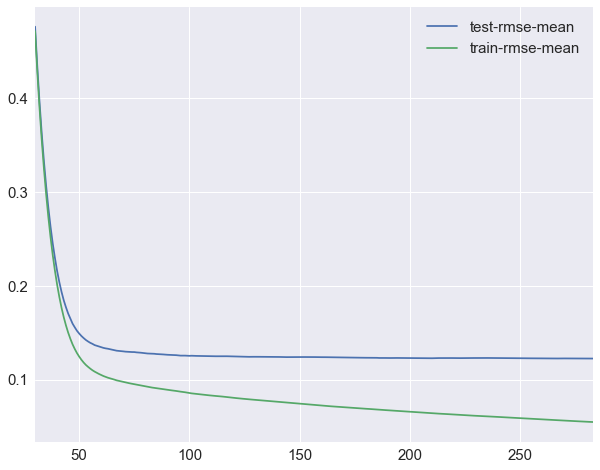
As you can see we stopped before reaching the maximum number of boosting rounds, that’s because after the 284th tree, adding more rounds did not lead to improvements of RMSE on the test dataset.
#xgb_reg = xgb.XGBRegressor(**our_params)
final_gb = xgb.train(our_params, xgdmat, num_boost_round = 284)
%matplotlib inline
import seaborn as sns
sns.set(font_scale = 1.5)
sorted(final_gb.get_fscore().items())
[('1stFlrSF', 122),
 ('2ndFlrSF', 39),
 ('3SsnPorch', 5),
 ('Alley_NA', 4),
 ('Alley_Pave', 10),
 ('BedroomAbvGr', 24),
 ('BldgType_2fmCon', 2),
 ('BldgType_Duplex', 1),
 ('BsmtCond', 11),
 ('BsmtExposure', 16),
 ('BsmtFinSF1', 67),
 ('BsmtFinSF2', 17),
 ('BsmtFinType1', 12),
 ('BsmtFinType2', 6),
 ('BsmtFullBath', 19),
 ('BsmtHalfBath', 3),
 ('BsmtQual', 11),
 ('BsmtUnfSF', 77),
 ('CentralAir_Y', 13),
 ('Condition1_Feedr', 3),
 ('Condition1_Norm', 19),
 ('Condition1_PosA', 1),
 ('Condition1_PosN', 3),
 ('Condition1_RRAe', 5),
 ('Condition1_RRAn', 1),
 ('Electrical_FuseF', 2),
 ('Electrical_SBrkr', 4),
 ('EnclosedPorch', 39),
 ('ExterCond', 17),
 ('ExterQual', 3),
 ('Exterior1st_2', 5),
 ('Exterior1st_3', 11),
 ('Exterior1st_4', 2),
 ('Exterior2nd_1', 10),
 ('Exterior2nd_2', 1),
 ('Exterior2nd_3', 1),
 ('Fence_GdWo', 8),
 ('Fence_MnPrv', 2),
 ('Fence_NA', 4),
 ('FireplaceQu', 8),
 ('Fireplaces', 4),
 ('Foundation_CBlock', 1),
 ('Foundation_PConc', 8),
 ('Foundation_Wood', 3),
 ('FullBath', 8),
 ('Functional', 31),
 ('GarageArea', 70),
 ('GarageCars', 8),
 ('GarageCond', 4),
 ('GarageFinish_RFn', 2),
 ('GarageFinish_Unf', 5),
 ('GarageQual', 5),
 ('GarageType_Attchd', 12),
 ('GarageType_Basment', 2),
 ('GarageType_BuiltIn', 1),
 ('GarageType_CarPort', 1),
 ('GarageType_Detchd', 4),
 ('GarageYrBlt', 56),
 ('GrLivArea', 116),
 ('HalfBath', 7),
 ('HeatingQC', 10),
 ('Heating_GasA', 3),
 ('Heating_Grav', 1),
 ('HouseStyle_1Story', 4),
 ('HouseStyle_2.5Unf', 2),
 ('HouseStyle_2Story', 1),
 ('HouseStyle_SLvl', 2),
 ('KitchenAbvGr', 8),
 ('KitchenQual', 20),
 ('LandContour_HLS', 1),
 ('LandContour_Low', 1),
 ('LandContour_Lvl', 5),
 ('LandSlope_Mod', 2),
 ('LandSlope_Sev', 1),
 ('LotArea', 102),
 ('LotConfig_CulDSac', 8),
 ('LotConfig_FR2', 4),
 ('LotConfig_FR3', 1),
 ('LotConfig_Inside', 5),
 ('LotFrontage', 52),
 ('LotShape_Reg', 2),
 ('LowQualFinSF', 7),
 ('MSSubClass_class2', 5),
 ('MSSubClass_class5', 7),
 ('MSSubClass_class6', 4),
 ('MSSubClass_class7', 1),
 ('MSSubClass_class8', 1),
 ('MSSubClass_class9', 1),
 ('MSZoning_FV', 2),
 ('MSZoning_RH', 1),
 ('MSZoning_RL', 5),
 ('MSZoning_RM', 5),
 ('MasVnrArea', 17),
 ('MasVnrType_BrkFace', 3),
 ('MasVnrType_Stone', 1),
 ('MiscVal', 3),
 ('Neighborhood_1', 4),
 ('Neighborhood_2', 7),
 ('Neighborhood_3', 10),
 ('Neighborhood_4', 8),
 ('OpenPorchSF', 38),
 ('OverallCond', 52),
 ('OverallQual', 68),
 ('PavedDrive_P', 1),
 ('PavedDrive_Y', 7),
 ('PoolArea', 8),
 ('RoofMatl_CompShg', 1),
 ('RoofMatl_Tar&Grv', 1),
 ('RoofMatl_WdShngl', 4),
 ('RoofStyle_Gable', 2),
 ('RoofStyle_Gambrel', 7),
 ('RoofStyle_Hip', 2),
 ('SaleCondition_Alloca', 5),
 ('SaleCondition_Family', 13),
 ('SaleCondition_Normal', 23),
 ('SaleCondition_Partial', 9),
 ('SaleType_ConLI', 1),
 ('SaleType_New', 9),
 ('SaleType_WD', 3),
 ('ScreenPorch', 22),
 ('Street_Pave', 9),
 ('TotRmsAbvGrd', 11),
 ('TotalBsmtSF', 62),
 ('WoodDeckSF', 37),
 ('YearBuilt', 65),
 ('YearRemodAdd', 42),
 ('YrSold', 19)]
##xgb.plot_importance(final_gb,max_num_features=50)
fig, ax = plt.subplots(figsize=(12,18))
#xgb.plot_importance(final_gb, max_num_features=50, height=0.8, ax=ax)
#plt.show()
%matplotlib inline
max_x=10
xgb.plot_importance(dict(sorted(final_gb.get_fscore().items(), reverse = True, key=lambda x:x[1])[:max_x]), height = 0.8)
<matplotlib.axes._subplots.AxesSubplot at 0x210fbb01240>
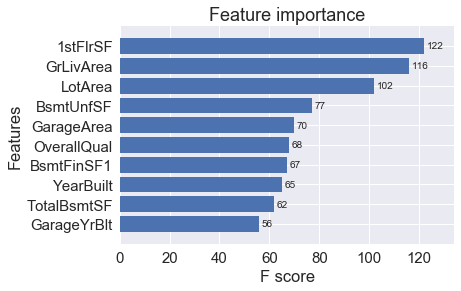
Now that we have an understanding of the feature importances, we can at least figure out better what is driving the splits most for the trees and where we may be able to make some improvements in feature engineering if possible. You can try playing around with the hyperparameters yourself or engineer some new features to see if you can beat the current benchmarks
The model has now been tuned using cross-validation grid search through the sklearn API and early stopping through the built-in XGBoost API. Now, we can see how it finally performs on the test set.
testdmat = xgb.DMatrix(X_test)
y_pred = final_gb.predict(testdmat) # Predict using our testdmat
y_pred
array([ 11.73430061,  11.97035789,  12.14089966, ...,  12.00389957,
        11.66779327,  12.29656219], dtype=float32)
y_pred = np.exp(y_pred)

output = pd.DataFrame({'Id': test_df['Id'], 'SalePrice': y_pred})
output.to_csv('prediction-ensemble.csv', index=False)
As we can see
#cv_xgb.shape
#print("Best MAE: {:.2f} with {} rounds".format(
#                 model.best_score,
#                 model.best_iteration+1))
#from xgboost import XGBRegressor
#xgb = XGBRegressor()
#xgb.fit(X_train, y_train)
#print(xgb.booster().get_score())
#imp = pd.DataFrame(xgb.feature_importances_ ,columns = ['Importance'],index = X_train.columns)
#imp = pd.DataFrame(xgb.booster().get_score(),index = X_train.columns)
#imp = imp.sort_values(['Importance'], ascending = False)
#model.booster().get_score(importance_type='weight')
#print(imp)