NumPy - Numerical & Scientific Computing with Python.
import numpy as np
import pandas as pd
import matplotlib.pyplot as plt
%matplotlib inline
Numpy
np.__version__
'1.12.1'
Representing any data as array of nos
No matter what the data are, the first step in making them analyzable will be to transform them into arrays of numbers For this reason, efficient storage and manipulation of numerical arrays is absolutely fundamental to the process of doing data science.
Enter numpy and pandas
NumPy (short for Numerical Python) provides an efficient interface to store and operate on dense data buffers. In some ways, NumPy arrays are like Python’s built-in list type, but NumPy arrays provide much more efficient storage and data operations as the arrays grow larger in size
Understanding Data Types in Python
in C, the data types of each variable are explicitly declared, while in Python the types are dynamically inferred. i.e)Python is dynamically typed wherease C is static type language.
This sort of flexibility is one piece that makes Python and other dynamically typed languages convenient and easy to use. Understanding how this works is an important piece of learning to analyze data efficiently and effectively with Python. But what this type flexibility also points to is the fact that Python variables are more than just their value; they also contain extra information about the type of the value.
A single integer in Python 3.4 actually contains four pieces:
ob_refcnt, a reference count that helps Python silently handle memory allocation and deallocation
ob_type, which encodes the type of the variable
ob_size, which specifies the size of the following data members
ob_digit, which contains the actual integer value that we expect thePython variable to represent
This means that there is some overhead in storing an integer in Python as compared to an integer in a compiled language like C
How are variables and memory managed in Python.
Automagically! No, really, you just create an object and the Python Virtual Machine handles the memory needed and where it shall be placed in the memory layout.
Does it have a stack and a heap and what algorithm is used to manage memory?
When we are talking about CPython it uses a private heap for storing objects. From the official Python documentation:
Memory management in Python involves a private heap containing all Python objects and data structures. The management of this private heap is ensured internally by the Python memory manager. The Python memory manager has different components which deal with various dynamic storage management aspects, like sharing, segmentation, preallocation or caching.
The algorithm used for garbage collecting is called Reference counting. That is the Python VM keeps an internal journal of how many references refer to an object, and automatically garbage collects it when there are no more references refering to it.
List Python data structure that holds many Python objects
Because of Python’s dynamic typing, we can even create heterogeneous lists
L3 = [True, "2", 3.0, 4]
[type(item) for item in L3]
[bool, str, float, int]
Fixed-type NumPy-style arrays lack this flexibility, but are much more efficient for storing and manipulating data.
While Python’s array object provides efficient storage of array-based data, NumPy adds to this efficient operations on that data.
NumPy is constrained to arrays that all contain the same type.will upcast if possible (here, integers are upcast to floating point):
##Creating numpy array from list
np.array([1, 4, 2, 5, 3])
array([1, 4, 2, 5, 3])
##numpy type upcast
np.array([3.14, 4, 2, 3])
array([ 3.14, 4. , 2. , 3. ])
##Set datatype explicitly
np.array([1, 2, 3, 4], dtype='float32')
array([ 1., 2., 3., 4.], dtype=float32)
# nested lists result in multidimensional arrays(unlike lists)
np.array([range(i, i + 3) for i in [2, 4, 6]])
array([[2, 3, 4],
       [4, 5, 6],
       [6, 7, 8]])
Creatin np arrays from scratch
Especially for larger arrays, it is more efficient to create arrays from scratch using routines built into NumPy. Here are several examples:
# Create a length-10 integer array filled with zeros
np.zeros(10, dtype=int)
array([0, 0, 0, 0, 0, 0, 0, 0, 0, 0])
# Create a 3x5 floating-point array filled with 1s
np.ones((3, 5), dtype=float)
array([[ 1.,  1.,  1.,  1.,  1.],
       [ 1.,  1.,  1.,  1.,  1.],
       [ 1.,  1.,  1.,  1.,  1.]])
# Create a 3x5 array filled with 3.14
np.full((3, 5), 3.14)
array([[ 3.14,  3.14,  3.14,  3.14,  3.14],
       [ 3.14,  3.14,  3.14,  3.14,  3.14],
       [ 3.14,  3.14,  3.14,  3.14,  3.14]])
# Create an array filled with a linear sequence
# Starting at 0, ending at 20, stepping by 2
# (this is similar to the built-in range() function)
np.arange(0, 20, 2)
array([ 0, 2, 4, 6, 8, 10, 12, 14, 16, 18])
# Create an array of five values evenly spaced between 0 and 1
np.linspace(0,1,5)
array([ 0. , 0.25, 0.5 , 0.75, 1. ])
# Create a 3x3 array of uniformly distributed
# random values between 0 and 1
np.random.random((3, 3))
array([[ 0.40890027,  0.5023264 ,  0.51346632],
       [ 0.82751189,  0.35064297,  0.12419154],
       [ 0.15690959,  0.63019322,  0.21561475]])
# Create a 3x3 array of normally distributed random values
# with mean 0 and standard deviation 1
np.random.normal(0, 1, (3, 3))
array([[-0.41040525, -0.39695729,  0.42291954],
       [-0.52527074,  0.54233525,  1.48757686],
       [-1.08965837, -0.45944806,  2.55026719]])
# Create a 3x3 array of random integers in the interval [0, 10)
np.random.randint(0, 10, (3, 3))
array([[8, 0, 1],
       [9, 2, 2],
       [8, 1, 7]])
# Create a 3x3 identity matrix
np.eye(3)
array([[ 1.,  0.,  0.],
       [ 0.,  1.,  0.],
       [ 0.,  0.,  1.]])
numpy dtype
Because NumPy is built in C, the types will be familiar to users of C, Fortran, and other related languages. bool_,int8,int16,int32,int64,uint(8,16,32,64),float(8,16,32,64),complex64(128)
np.random.seed(0)  # seed for reproducibility
x1 = np.random.randint(10, size=6)  # One-dimensional array
x2 = np.random.randint(10, size=(3, 4))  # Two-dimensional array
x3 = np.random.randint(10, size=(3, 4, 5))  # Three-dimensional array
print("x3 ndim: ", x3.ndim)
print("x3 shape:", x3.shape)
print("x3 size: ", x3.size)
x3 ndim:  3
x3 shape: (3, 4, 5)
x3 size:  60
print("dtype:", x3.dtype)
dtype: int32
print("itemsize:", x3.itemsize, "bytes")  ##which lists the size (in bytes) of each array element
print("nbytes:", x3.nbytes, "bytes")  ##which lists the total size (in bytes) of the array
itemsize: 4 bytes
nbytes: 240 bytes
x1[0],x1[4],x1[-1],x1[-2]
(5, 7, 9, 7)
x2[0,0],x2[2,0],x2[2,-1]
(3, 1, 7)
Array Slicing: Accessing Subarrays
x[start:stop:step]
x1[:5]
array([5, 0, 3, 3, 7])
x1[1:4]
array([0, 3, 3])
x1[::2] # every other element
array([5, 3, 7])
x1[1::2] # every other element, starting at index 1
array([0, 3, 9])
A potentially confusing case is when the step value is negative. In this case, the defaults for start and stop are swapped. This becomes a convenient way to reverse an array:
x1[::-1] # all elements, reversed
array([9, 7, 3, 3, 0, 5])
x1[5::-2] # reversed every other from index 5
array([9, 3, 0])
x2[:2, :3] # two rows, three columns
array([[3, 5, 2],
       [7, 6, 8]])
x2[:3, ::2] # all rows, every other column
array([[3, 2],
       [7, 8],
       [1, 7]])
x2[::-1, ::-1] #subarray dimensions can even be reversed together
array([[7, 7, 6, 1],
       [8, 8, 6, 7],
       [4, 2, 5, 3]])
One important—and extremely useful—thing to know about array slices is that they return views rather than copies of the array data. This is one area in which NumPy array slicing differs from Python list slicing: in lists, slices will be copies.
x2_sub_copy = x2[:2, :2].copy() ###use this instead when manipulating subarrays
print(x2_sub_copy)
[[3 5]
 [7 6]]
Reshaping of Arrays
grid = np.arange(1, 10).reshape((3, 3))
print(grid)
[[1 2 3]
 [4 5 6]
 [7 8 9]]
Another common reshaping pattern is the conversion of a one-dimensional array into a two-dimensional row or column matrix. You can do this with the reshape method, or more easily by making use of the newaxis keyword within a slice operation:
x = np.array([1, 2, 3])
# row vector via reshape
x.reshape((1, 3))
array([[1, 2, 3]])
# row vector via newaxis
x[np.newaxis, :]
array([[1, 2, 3]])
# column vector via reshape
x.reshape((3, 1))
array([[1],
       [2],
       [3]])
# column vector via newaxis
x[:, np.newaxis]
array([[1],
       [2],
       [3]])
Array Concatenation and Splitting
Concatenation, or joining of two arrays in NumPy np.concatenate, np.vstack, and np.hstack. np.concatenate takes a tuple or list of arrays as its first argument
x = np.array([1, 2, 3])
y = np.array([3, 2, 1])
np.concatenate([x, y])
array([1, 2, 3, 3, 2, 1])
z = [99, 99, 99]
print(np.concatenate([x, y, z]))
[ 1 2 3 3 2 1 99 99 99]
grid = np.array([[1, 2, 3],
                [4, 5, 6]])
# concatenate along the first axis
np.concatenate([grid, grid])
array([[1, 2, 3],
       [4, 5, 6],
       [1, 2, 3],
       [4, 5, 6]])
# concatenate along the second axis (zero-indexed)
np.concatenate([grid, grid], axis=1)
array([[1, 2, 3, 1, 2, 3],
       [4, 5, 6, 4, 5, 6]])
For working with arrays of mixed dimensions, it can be clearer to use the np.vstack (vertical stack) and np.hstack (horizontal stack) functions:
x = np.array([1, 2, 3])
grid = np.array([[9, 8, 7],
                [6, 5, 4]])
# vertically stack the arrays
np.vstack([x, grid])
array([[1, 2, 3],
       [9, 8, 7],
       [6, 5, 4]])
# horizontally stack the arrays
y = np.array([[99],
             [99]])
np.hstack([grid, y])
array([[ 9,  8,  7, 99],
       [ 6,  5,  4, 99]])
SPLITTING OF ARRAYS
np.split, np.hsplit, and np.vsplit. For each of these, we can pass a list of indices giving the split points
x = [1, 2, 3, 99, 99, 3, 2, 1]
x1,x2,x3=np.split(x,[3,5])
print(x1,x2,x3)
[1 2 3] [99 99] [3 2 1]
grid=np.arange(16).reshape([4,4])
grid
array([[ 0,  1,  2,  3],
       [ 4,  5,  6,  7],
       [ 8,  9, 10, 11],
       [12, 13, 14, 15]])
upper,lower=np.vsplit(grid,[2])
print(upper,"\n\n",lower)
[[0 1 2 3]
 [4 5 6 7]]

 [[ 8  9 10 11]
 [12 13 14 15]]
left,right=np.hsplit(grid,[2])
print(left,"\n\n",right)
[[ 0  1]
 [ 4  5]
 [ 8  9]
 [12 13]]

 [[ 2  3]
 [ 6  7]
 [10 11]
 [14 15]]
Computation on NumPy Arrays: Universal Functions
Computation on NumPy arrays - fast vectorized operation - generally implemented through Numpy’s universal funcs (Ufuncs) - which can be used to make repeated calculations on array elements much more efficient
import numpy as np
np.random.seed(0)

def ComputeRec(values):
    array=np.empty(len(values))
    for i in range(len(values)):
        array[i]=1/values[i]
    print(array)

v=np.random.randint(1,10,size=5)
ComputeRec(v)
[ 0.16666667 1. 0.25 0.25 0.125 ]
bigarray=np.random.randint(1,100,size=1000000)
%timeit ComputeRec(bigarray)
[ 0.1         0.01190476  0.04545455 ...,  0.01428571  0.01098901
  0.01149425]
[ 0.1         0.01190476  0.04545455 ...,  0.01428571  0.01098901
  0.01149425]
[ 0.1         0.01190476  0.04545455 ...,  0.01428571  0.01098901
  0.01149425]
[ 0.1         0.01190476  0.04545455 ...,  0.01428571  0.01098901
  0.01149425]
[ 0.1         0.01190476  0.04545455 ...,  0.01428571  0.01098901
  0.01149425]
[ 0.1         0.01190476  0.04545455 ...,  0.01428571  0.01098901
  0.01149425]
[ 0.1         0.01190476  0.04545455 ...,  0.01428571  0.01098901
  0.01149425]
[ 0.1         0.01190476  0.04545455 ...,  0.01428571  0.01098901
  0.01149425]
857 ms ± 23.4 ms per loop (mean ± std. dev. of 7 runs, 1 loop each)
slow operation comparitively because of the type-checking and function dispatches that CPython must do at each cycle of the loop.
Each time the reciprocal is computed, Python first examines the object’s type and does a dynamic lookup of the correct function to use for that type. If we were working in compiled code instead, this type specification would be known before the code executes and the result could be computed much more efficiently.
Introducing UFuncs
For many types of operations, NumPy provides a convenient interface into just this kind of statically typed, compiled routine. This is known as a vectorized operation. You can accomplish this by simply performing an operation on the array, which will then be applied to each element. This vectorized approach is designed to push the loop into the compiled layer that underlies NumPy, leading to much faster execution.
All of these arithmetic operations are simply convenient wrappers around specific functions built into NumPy; for example, the + operator is a wrapper for the add function: np.add(x, 2) == x+2
x = np.array([3 - 4j, 4 - 3j, 2 + 0j, 0 + 1j])
np.abs(x)
array([ 5., 5., 2., 1.])
TRIGONOMETRIC FUNCTIONS
NumPy provides a large number of useful ufuncs, and some of the mostuseful for the data scientist are the trigonometric functions. We’llstart by defining an array of angles:
theta = np.linspace(0,np.pi,3)
print("theta      = ", theta)
print("sin(theta) = ", np.sin(theta))
print("cos(theta) = ", np.cos(theta))
print("tan(theta) = ", np.tan(theta))
theta      =  [ 0.          1.57079633  3.14159265]
sin(theta) =  [  0.00000000e+00   1.00000000e+00   1.22464680e-16]
cos(theta) =  [  1.00000000e+00   6.12323400e-17  -1.00000000e+00]
tan(theta) =  [  0.00000000e+00   1.63312394e+16  -1.22464680e-16]
####Inverse trigonometric functions
x = [-1, 0, 1]
print("x         = ", x)
print("arcsin(x) = ", np.arcsin(x))
print("arccos(x) = ", np.arccos(x))
print("arctan(x) = ", np.arctan(x))
x         =  [-1, 0, 1]
arcsin(x) =  [-1.57079633  0.          1.57079633]
arccos(x) =  [ 3.14159265  1.57079633  0.        ]
arctan(x) =  [-0.78539816  0.          0.78539816]
EXPONENTS AND LOGARITHMS
x = [1, 2, 3]
print("x     =", x)
print("e^x   =", np.exp(x))
print("2^x   =", np.exp2(x))
print("3^x   =", np.power(3, x))
x     = [1, 2, 3]
e^x   = [  2.71828183   7.3890561   20.08553692]
2^x   = [ 2.  4.  8.]
3^x   = [ 3  9 27]
#### The inverse of the exponentials, the logarithms, are also available
x = [1, 2, 4, 10]
print("x        =", x)
print("ln(x)    =", np.log(x))
print("log2(x)  =", np.log2(x))
print("log10(x) =", np.log10(x))
x        = [1, 2, 4, 10]
ln(x)    = [ 0.          0.69314718  1.38629436  2.30258509]
log2(x)  = [ 0.          1.          2.          3.32192809]
log10(x) = [ 0.          0.30103     0.60205999  1.        ]
#### specialized versions that are useful formaintaining precision with very small input
x = [0, 0.001, 0.01, 0.1]
print("exp(x) - 1 =", np.expm1(x))
print("log(1 + x) =", np.log1p(x))
exp(x) - 1 = [ 0.          0.0010005   0.01005017  0.10517092]
log(1 + x) = [ 0.          0.0009995   0.00995033  0.09531018]
Specialized ufuncs
NumPy has many more ufuncs available, including hyperbolic trigfunctions, bitwise arithmetic, comparison operators, conversions fromradians to degrees, rounding and remainders, and much more. A lookthrough the NumPy documentation reveals a lot of interestingfunctionality.Another excellent source for more specialized and obscure ufuncs is the submodule scipy.special. If you want to compute some obscuremathematical function on your data, chances are it is implemented in #### scipy.special. There are far too many functions to list them all,but the following snippet shows a couple that might come up in a statistics context:
from scipy import special
# Gamma functions (generalized factorials) and related functions
x = [1, 5, 10]
print("gamma(x)     =", special.gamma(x))
print("ln|gamma(x)| =", special.gammaln(x))
print("beta(x, 2)   =", special.beta(x, 2))
gamma(x)     = [  1.00000000e+00   2.40000000e+01   3.62880000e+05]
ln|gamma(x)| = [  0.           3.17805383  12.80182748]
beta(x, 2)   = [ 0.5         0.03333333  0.00909091]
# Error function (integral of Gaussian)
# its complement, and its inverse
x = np.array([0, 0.3, 0.7, 1.0])
print("erf(x)  =", special.erf(x))
print("erfc(x) =", special.erfc(x))
print("erfinv(x) =", special.erfinv(x))
erf(x)  = [ 0.          0.32862676  0.67780119  0.84270079]
erfc(x) = [ 1.          0.67137324  0.32219881  0.15729921]
erfinv(x) = [ 0.          0.27246271  0.73286908         inf]
Advanced UFunc features
##SPECIFYING OUTPUT
x=np.random.randint(1,10,5)
y=np.empty_like(x)
np.multiply(x,2,out=y)
print(x,y)
[3 6 4 2 7] [ 6 12 8 4 14]
#If we had instead written y[::2] = 2 ** x, this would have resulted in the creation of a temporary array
#to hold the results of 2 ** x, followed by a second operation copying those values into the y array.
#This doesn’t make much of a difference for such a small computation, but for very large arrays the memory savings
#from careful use of the out argument can be significant.
y=np.zeros(10)
np.power(2,x,out=y[::2])
print(y)
[ 8. 0. 64. 0. 16. 0. 4. 0. 128. 0.]
##AGGREGATES
#Reduce array with particular operation
x = np.arange(1,6)
print(np.add.reduce(x))
print(np.multiply.reduce(x))
#store all the intermediate results of the computation,use accumulate
print(np.multiply.accumulate(x))

#Note that for these particular cases, there are dedicated NumPy functions
#to compute the results (np.sum, np.prod, np.cumsum, np.cumprod)
15
120
[  1   2   6  24 120]
##OUTER PRODUCTS
x=np.arange(1,6)
np.multiply.outer(x,x)
array([[ 1,  2,  3,  4,  5],
       [ 2,  4,  6,  8, 10],
       [ 3,  6,  9, 12, 15],
       [ 4,  8, 12, 16, 20],
       [ 5, 10, 15, 20, 25]])
Aggregations: Min, Max, and Everything in Between
summary statistics for the data - useful
L = np.random.random(100)
np.sum(L)
#However, because it executes the operation in compiled code, NumPy’s version
#of the operation is computed much more quickly:
51.672948923416811
#Minimum and Maximum
big_array = np.random.rand(1000000)
%timeit sum(big_array)
%timeit np.sum(big_array)
327 ms ± 3.96 ms per loop (mean ± std. dev. of 7 runs, 1 loop each)
2.7 ms ± 92.1 µs per loop (mean ± std. dev. of 7 runs, 100 loops each)
np.min(big_array), np.max(big_array)
(7.0712031718933588e-07, 0.99999972076563337)
print(big_array.min(), big_array.max(), big_array.sum()) ##shorter syntax
7.07120317189e-07 0.999999720766 500216.268061
MULTIDIMENSIONAL AGGREGATES
Aggregation functions take an additional argument specifying the axis along which the aggregate is computed. For example, we can find the minimum value within each column by specifying axis=0:
M = np.random.random((3, 4))
print(M)
M.min()
[[ 0.18441813  0.71417358  0.76371195  0.11957117]
 [ 0.37578601  0.11936151  0.37497044  0.22944653]
 [ 0.07452786  0.41843762  0.99939192  0.66974416]]


0.074527862651998289
M.min(axis=0)
array([ 0.07452786, 0.11936151, 0.37497044, 0.11957117])
M.max(axis=1)
array([ 0.76371195, 0.37578601, 0.99939192])
OTHER AGGREGATION FUNCTIONS
NumPy provides many other aggregation functions, but we won’t discuss them in detail here. Additionally, most aggregates have a NaN-safe counterpart that computes the result while ignoring missing values, which are marked by the special IEEE floating-point NaN value
Function Name	NaN-safe Version
np.sum          np.nansum
np.prod         np.nanprod
np.mean         np.nanmean
np.std          np.nanstd
np.var          np.nanvar
np.min          np.nanmin
np.max          np.nanmax
np.argmin       np.nanargmin
np.argmax       np.nanargmax
np.median       np.nanmedian
np.percentile   np.nanpercentile
np.any          N/A
np.all          N/A
Computation on Arrays: Broadcasting
NumPy’s universal functions can be used to vectorize operations and thereby remove slow Python loops. Another means of vectorizing operations is to use NumPy’s broadcasting functionality. Broadcasting is simply a set of rules for applying binary ufuncs (addition, subtraction, multiplication, etc.) on arrays of different sizes.
Rules of Broadcasting Broadcasting in NumPy follows a strict set of rules to determine the interaction between the two arrays:
Rule 1: If the two arrays differ in their number of dimensions, the shape of the one with fewer dimensions is padded with ones on its leading (left) side.
Rule 2: If the shape of the two arrays does not match in any dimension, the array with shape equal to 1 in that dimension is stretched to match the other shape.
Rule 3: If in any dimension the sizes disagree and neither is equal to 1, an error is raised.
To make these rules clear, let’s consider a few examples in detail.
CENTERING AN ARRAY
In the previous section, we saw that ufuncs allow a NumPy user to remove the need to explicitly write slow Python loops. Broadcasting extends this ability. One commonly seen example is centering an array of data. Imagine you have an array of 10 observations, each of which consists of 3 values. Using the standard convention (see “Data Representation in Scikit-Learn”), we’ll store this in a 10×3 array:
X = np.random.random((10, 3))
X
array([[ 0.54717434,  0.82711104,  0.23097044],
       [ 0.16283152,  0.27950484,  0.58540569],
       [ 0.90657413,  0.18671025,  0.07262851],
       [ 0.0068539 ,  0.07533272,  0.77114754],
       [ 0.94502816,  0.79396332,  0.81250458],
       [ 0.68306202,  0.09142216,  0.72943166],
       [ 0.49977781,  0.88075176,  0.77188336],
       [ 0.33609389,  0.35670153,  0.26486376],
       [ 0.51351043,  0.18439926,  0.90137772],
       [ 0.75292208,  0.26398243,  0.46383154]])
#We can compute the mean of each feature using the mean aggregate across the first dimension:
Xmean=X.mean(axis=0)
Xmean
array([ 0.53538283, 0.39398793, 0.56040448])
#And now we can center the X array by subtracting the mean (this is a broadcasting operation):
X_centered=X-Xmean
X
array([[ 0.54717434,  0.82711104,  0.23097044],
       [ 0.16283152,  0.27950484,  0.58540569],
       [ 0.90657413,  0.18671025,  0.07262851],
       [ 0.0068539 ,  0.07533272,  0.77114754],
       [ 0.94502816,  0.79396332,  0.81250458],
       [ 0.68306202,  0.09142216,  0.72943166],
       [ 0.49977781,  0.88075176,  0.77188336],
       [ 0.33609389,  0.35670153,  0.26486376],
       [ 0.51351043,  0.18439926,  0.90137772],
       [ 0.75292208,  0.26398243,  0.46383154]])
X_centered.mean(0) ##all values equal to zero
array([ 9.99200722e-17, 0.00000000e+00, 1.22124533e-16])
Comparisons, Masks, and Boolean Logic
Boolean masks to examine and manipulate values within NumPy arrays. Masking comes up when you want to extract, modify, count, or otherwise manipulate values in an array based on some criterion: for example, you might wish to count all values greater than a certain value, or perhaps remove all outliers that are above some threshold. In NumPy, Boolean masking is often the most efficient way to accomplish these types of tasks.
x = np.array([1, 2, 3, 4, 5])
x<3
array([ True, True, False, False, False], dtype=bool)
x[x<3]
array([1, 2])
x[x!=3]
array([1, 2, 4, 5])
COUNTING ENTRIES
rng = np.random.RandomState(0)
x = rng.randint(10, size=(3, 4))
# how many values less than 6?
np.count_nonzero(x < 6)
8
#Another way to get at this information is to use np.sum; in this case,
#False is interpreted as 0, and True is interpreted as 1:
np.sum(x < 6)
8
# how many values less than 6 in each row?
np.sum(x < 6, axis=0)
array([2, 2, 2, 2])
#If we’re interested in quickly checking whether any or all the values are true,
#we can use (you guessed it) np.any() or np.all():
# are there any values greater than 8?
np.any(x > 8)
True
# are there any values less than zero?
np.any(x < 0)
False
# are all values less than 10?
np.all(x < 10)
True
# are all values equal to 6?
np.all(x==6)
False
# are all values in each row less than 8?
np.all(x < 8, axis=1)
array([ True, False, True], dtype=bool)
BOOLEAN OPERATORS
We’ve already seen how we might count, say, all days with rain less than four inches, or all days with rain greater than two inches. But what if we want to know about all days with rain less than four inches and greater than one inch? This is accomplished through Python’s bitwise logic operators, &, |, ^, and ~. Like with the standard arithmetic operators, NumPy overloads these as ufuncs that work element-wise on (usually Boolean) arrays.
For example, we can address this sort of compound question as follows:
>rainfall = pd.read_csv('data/Seattle2014.csv')['PRCP'].values
>inches = rainfall / 254  # 1/10mm -> inches
>inches.shape
>np.sum((inches > 0.5) & (inches < 1)) ####### Out[1] 29
>np.sum(~( (inches <= 0.5) | (inches >= 1) )) ###### Out[2] 29
>print("Number days without rain:      ", np.sum(inches == 0))
>print("Number days with rain:         ", np.sum(inches != 0))
>print("Days with more than 0.5 inches:", np.sum(inches > 0.5))
>print("Rainy days with < 0.1 inches  :", np.sum((inches > 0) & (inches < 0.2)))
Boolean Arrays as Masks
#construct a mask of all rainy days
rainy = (inches > 0)

#construct a mask of all summer days (June 21st is the 172nd day)
summer = (np.arange(365) - 172 < 90) & (np.arange(365) - 172 > 0)

print("Median precip on rainy days in 2014 (inches):   ",np.median(inches[rainy]))
print("Median precip on summer days in 2014 (inches):  ",np.median(inches[summer]))
print("Maximum precip on summer days in 2014 (inches): ",np.max(inches[summer]))
print("Median precip on non-summer rainy days (inches):",np.median(inches[rainy & ~summer]))
Fancy Indexing
Fancy indexing is conceptually simple: it means passing an array of indices to access multiple array elements at once Fancy indexing is like the simple indexing we’ve already seen, but we pass arrays of indices in place of single scalars. This allows us to very quickly access and modify complicated subsets of an array’s values.
rand = np.random.RandomState(42)
x=rand.randint(100,size=10)
print(x)
[51 92 14 71 60 20 82 86 74 74]
[x[3], x[7], x[2]]
[71, 86, 14]
ind = [3, 7, 4]
x[ind]
array([71, 86, 60])
#With fancy indexing, the shape of the result reflects the shape of the index arrays rather than the shape of the array being indexed:
ind=np.array([[3,7],
             [4,5]])
x[ind]
array([[71, 86],
       [60, 20]])
#Fancy indexing also works in multiple dimensions. Consider the following array:
x=np.arange(12).reshape((3,4))
x
array([[ 0,  1,  2,  3],
       [ 4,  5,  6,  7],
       [ 8,  9, 10, 11]])
row=np.array([0,1,2])
col=np.array([2,1,3])
x[row,col]
##X[0, 2], the second is X[1, 1], and the third is X[2, 3]
array([ 2, 5, 11])
x[row[:, np.newaxis], col]
array([[ 2,  1,  3],
       [ 6,  5,  7],
       [10,  9, 11]])
row[:, np.newaxis] * col
#It is always important to remember with fancy indexing that the returnvalue reflects the broadcasted shape of the indices, rather than theshape of the array being indexed.
array([[0, 0, 0],
       [2, 1, 3],
       [4, 2, 6]])
Combined Indexing
For even more powerful operations, fancy indexing can be combined with the other indexing schemes we’ve seen:
X=np.arange(0,12).reshape((3,4))
X
array([[ 0,  1,  2,  3],
       [ 4,  5,  6,  7],
       [ 8,  9, 10, 11]])
X[2,[2,0,1]] ##combine fancy indexing with simple indices
array([10, 8, 9])
X[1:,[2,0,1]] ## combine fancy indexing with slicing
array([[ 6,  4,  5],
       [10,  8,  9]])
mask = np.array([1, 0, 1, 0], dtype=bool) ##combine fancy indexing with masking
X[row[:, np.newaxis], mask]
array([[ 0,  2],
       [ 4,  6],
       [ 8, 10]])
Modifying Values with Fancy Indexing
Just as fancy indexing can be used to access parts of an array, it can also be used to modify parts of an array. For example, imagine we have an array of indices and we’d like to set the corresponding items in an array to some value:
x = np.arange(10)
i = np.array([2, 1, 8, 4])
x[i] = 99
print(x)
[ 0 99 99 3 99 5 6 7 99 9]
x[i] -= 10
print(x)
[ 0 89 89 3 89 5 6 7 89 9]
j=np.array([2,5,7])
x[j]+=150
print(x)
[ 0 89 239 3 89 155 6 157 89 9]
x =np.zeros(10)
x[[0,0]]=[4,6]
print(x)
[ 6. 0. 0. 0. 0. 0. 0. 0. 0. 0.]
i = [2, 3, 3, 4, 4, 4]
x[i]+=1  ### x[i] = x[i] + 1.
x
array([ 6., 0., 1., 1., 1., 0., 0., 0., 0., 0.])
x[i] + 1 is evaluated, and then the result is assigned to the indices in x. With this in mind, it is not the augmentation that happens multiple times, but the assignment, which leads to the rather nonintuitive results.
So what if you want the other behavior where the operation is repeated? For this, you can use the at() method of ufuncs (available since NumPy 1.8), and do the following:
#The at() method does an in-place application of the given operator at the specified indices (here, i)
#with the specified value (here, 1). Another method that is similar in spirit is the reduceat() method of ufuncs,
#which you can read about in the NumPy documentation.
x = np.zeros(10)
np.add.at(x, i, 1)
print(x)
[ 0. 0. 1. 2. 3. 0. 0. 0. 0. 0.]
##Example: Binning Data
np.random.seed(42)
x=np.random.randn(100)
#compute a histogram by hand
bins=np.linspace(-5,5,20)
counts=np.zeros_like(bins)
#find appropriate bin for each x
i=np.searchsorted(bins,x)
# add 1 to each of these bins
np.add.at(counts,i,1)
print(x)
print(bins)
[ 0.49671415 -0.1382643   0.64768854  1.52302986 -0.23415337 -0.23413696
  1.57921282  0.76743473 -0.46947439  0.54256004 -0.46341769 -0.46572975
  0.24196227 -1.91328024 -1.72491783 -0.56228753 -1.01283112  0.31424733
 -0.90802408 -1.4123037   1.46564877 -0.2257763   0.0675282  -1.42474819
 -0.54438272  0.11092259 -1.15099358  0.37569802 -0.60063869 -0.29169375
 -0.60170661  1.85227818 -0.01349722 -1.05771093  0.82254491 -1.22084365
  0.2088636  -1.95967012 -1.32818605  0.19686124  0.73846658  0.17136828
 -0.11564828 -0.3011037  -1.47852199 -0.71984421 -0.46063877  1.05712223
  0.34361829 -1.76304016  0.32408397 -0.38508228 -0.676922    0.61167629
  1.03099952  0.93128012 -0.83921752 -0.30921238  0.33126343  0.97554513
 -0.47917424 -0.18565898 -1.10633497 -1.19620662  0.81252582  1.35624003
 -0.07201012  1.0035329   0.36163603 -0.64511975  0.36139561  1.53803657
 -0.03582604  1.56464366 -2.6197451   0.8219025   0.08704707 -0.29900735
  0.09176078 -1.98756891 -0.21967189  0.35711257  1.47789404 -0.51827022
 -0.8084936  -0.50175704  0.91540212  0.32875111 -0.5297602   0.51326743
  0.09707755  0.96864499 -0.70205309 -0.32766215 -0.39210815 -1.46351495
  0.29612028  0.26105527  0.00511346 -0.23458713]
[-5.         -4.47368421 -3.94736842 -3.42105263 -2.89473684 -2.36842105
 -1.84210526 -1.31578947 -0.78947368 -0.26315789  0.26315789  0.78947368
  1.31578947  1.84210526  2.36842105  2.89473684  3.42105263  3.94736842
  4.47368421  5.        ]
plt.plot(bins,counts,linestyle='steps')
[<matplotlib.lines.Line2D at 0x287233f51d0>]
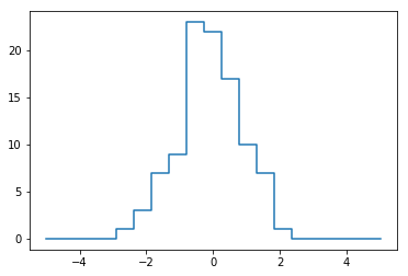
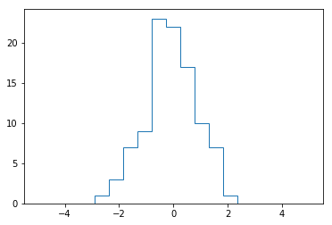
#Of course, it would be silly to have to do this each time you want to plot a histogram.
#This is why Matplotlib provides the plt.hist() routine, which does the same in a single line:

plt.hist(x, bins, histtype='step')
(array([  0.,   0.,   0.,   0.,   1.,   3.,   7.,   9.,  23.,  22.,  17.,
         10.,   7.,   1.,   0.,   0.,   0.,   0.,   0.]),
 array([-5.        , -4.47368421, -3.94736842, -3.42105263, -2.89473684,
        -2.36842105, -1.84210526, -1.31578947, -0.78947368, -0.26315789,
         0.26315789,  0.78947368,  1.31578947,  1.84210526,  2.36842105,
         2.89473684,  3.42105263,  3.94736842,  4.47368421,  5.        ]),
 <a list of 1 Patch objects>)
Sorting Arrays
Fast Sorting in NumPy: np.sort and np.argsort By default np.sort uses an script upper O left-bracket upper N log upper N right-bracket, quicksort algorithm, though mergesort and heapsort are also available. For most applications, the default quicksort is more than sufficient.
To return a sorted version of the array without modifying the input, you can use np.sort:
x = np.array([2, 1, 4, 3, 5])
np.sort(x)
array([1, 2, 3, 4, 5])
#If you prefer to sort the array in-place, you can instead use the sort method of arrays:
x.sort()
print(x)
[1 2 3 4 5]
#A related function is argsort, which instead returns the indices of the sorted elements:
x = np.array([2, 1, 4, 3, 5])
i = np.argsort(x)
print(i)
[1 0 3 2 4]
The first element of this result gives the index of the smallest element, the second value gives the index of the second smallest, and so on. These indices can then be used (via fancy indexing) to construct the sorted array if desired:
x[i]
array([1, 2, 3, 4, 5])
SORTING ALONG ROWS OR COLUMNS
A useful feature of NumPy’s sorting algorithms is the ability to sort along specific rows or columns of a multidimensional array using the axis argument. For example:
rand = np.random.RandomState(42)
X = rand.randint(0, 10, (4, 6))
print(X)
[[6 3 7 4 6 9]
 [2 6 7 4 3 7]
 [7 2 5 4 1 7]
 [5 1 4 0 9 5]]
# sort each column of X
np.sort(X, axis=0)
array([[2, 1, 4, 0, 1, 5],
       [5, 2, 5, 4, 3, 7],
       [6, 3, 7, 4, 6, 7],
       [7, 6, 7, 4, 9, 9]])
sort each row of X
np.sort(X, axis=1)
Keep in mind that this treats each row or column as an independent array, and any relationships between the row or column values will be lost!
Partial Sorts: Partitioning
Sometimes we’re not interested in sorting the entire array, but simply want to find the K smallest values in the array. NumPy provides this in the np.partition function. np.partition takes an array and a number K; the result is a new array with the smallest K values to the left of the partition, and the remaining values to the right, in arbitrary order:
x = np.array([7, 2, 3, 1, 6, 5, 4])
np.partition(x, 3)
array([2, 1, 3, 4, 6, 5, 7])
np.partition(X, 2, axis=1)
array([[3, 4, 6, 7, 6, 9],
       [2, 3, 4, 7, 6, 7],
       [1, 2, 4, 5, 7, 7],
       [0, 1, 4, 5, 9, 5]])
Finally, just as there is a np.argsort that computes indices of the sort, there is a np.argpartition that computes indices of the partition. We’ll see this in action in the following section.
Structured Data: NumPy’s Structured Arrays
NumPy’s structured arrays and record arrays, which provide efficient storage for compound, heterogeneous data. scenarios like this often lend themselves to the use of Pandas DataFrames
name = ['Alice', 'Bob', 'Cathy', 'Doug']
age = [25, 45, 37, 19]
weight = [55.0, 85.5, 68.0, 61.5]
data = np.zeros(4, dtype={'names':('name', 'age', 'weight'),
                                 'formats':('U10', 'i4', 'f8')})
print(data.dtype) ###U10 - Unicode string of maximum length 10## i4' translates to “4-byte (i.e., 32 bit)## f8' translates to “8-byte (i.e., 64 bit) float
[('name', '<U10'), ('age', '<i4'), ('weight', '<f8')]
data['name'] = name
data['age'] = age
data['weight'] = weight
print(data)
[('Alice', 25,  55. ) ('Bob', 45,  85.5) ('Cathy', 37,  68. )
 ('Doug', 19,  61.5)]
As we had hoped, the data is now arranged together in one convenient block of memory. The handy thing with structured arrays is that you can now refer to values either by index or by name:
# Get all names
data['name']
array(['Alice', 'Bob', 'Cathy', 'Doug'],
      dtype='<U10')
# Get first row of data
data[0]
('Alice', 25, 55.)
#Get the name from the last row
data[-1]['name']
'Doug'
# Get names where age is under 30
data[data['age'] < 30]['name']
array(['Alice', 'Doug'],
      dtype='<U10')
np.dtype({'names':('name', 'age', 'weight'),
                  'formats':((np.str_, 10), int, np.float32)})
dtype([('name', '<U10'), ('age', '<i4'), ('weight', '<f4')])
~~~~~~~~~~~~~~~~~~~~~~~~~~~~~~~~~~~~~~~~~~~~~~~~~~~~~~~~~~~~~~~~~~~~~~~~~~~~~~~~~~~~~~~~~~~~~~~~~~~~~~~~~~~~~~~~~~~~~
a=np.array([2,3,4,5,6,7,8,9])
b=[2,3,4,5,6,7,8,9]
%%timeit a1=list()
for i in b:
    a1.append(i*5)
2.2 µs ± 65.2 ns per loop (mean ± std. dev. of 7 runs, 100000 loops each)
%timeit b*5
367 ns ± 5.04 ns per loop (mean ± std. dev. of 7 runs, 1000000 loops each)
s=pd.Series([1,2,3,4,5,6,7])
s
0    1
1    2
2    3
3    4
4    5
5    6
6    7
dtype: int64
type(s.values)
numpy.ndarray
s1=pd.Series({'a':1,'b':2,'d':3})
s1.values
array([1, 2, 3], dtype=int64)
s1['a':'b']
a    1
b    2
dtype: int64
s1
a    1
b    2
d    3
dtype: int64
s2=pd.Series({'a':4,'b':5,'c':6})
df=pd.DataFrame({'s1':s1,'s2':s2})
df.fillna(0,inplace=True)
df.stack().mean()
3.5
df.replace('9',9,inplace=True)
df.stack().mean()
3.5
df.stack()['a']
s1    1.0
s2    4.0
dtype: float64
for row in df.stack():
    print(row)
1.0
4.0
2.0
5.0
6.0
3.0
df.stack()['a':'b']
a  s1    1.0
   s2    4.0
b  s1    2.0
   s2    5.0
dtype: float64
df
| s1 | s2 | |
|---|---|---|
| a | 1.0 | 4.0 |
| b | 2.0 | 5.0 |
| c | NaN | 6.0 |
| d | 3.0 | NaN |
for row in df.index:
    print(df.stack()[row].mean())
2.5
3.5
6.0
3.0
df.mean(axis=1)
a    2.5
b    3.5
c    6.0
d    3.0
dtype: float64
rng = np.random.RandomState(42)
df1=pd.DataFrame(rng.randint(0, 10, (3, 3)),
                         columns=list('BAC'))
df1
| B | A | C | |
|---|---|---|---|
| 0 | 6 | 3 | 7 |
| 1 | 4 | 6 | 9 |
| 2 | 2 | 6 | 7 |
df.add(df1,fill_value=5)
| A | B | C | s1 | s2 | |
|---|---|---|---|---|---|
| a | NaN | NaN | NaN | 6.0 | 9.0 |
| b | NaN | NaN | NaN | 7.0 | 10.0 |
| c | NaN | NaN | NaN | NaN | 11.0 |
| d | NaN | NaN | NaN | 8.0 | NaN |
| 0 | 8.0 | 11.0 | 12.0 | NaN | NaN |
| 1 | 11.0 | 9.0 | 14.0 | NaN | NaN |
| 2 | 11.0 | 7.0 | 12.0 | NaN | NaN |
df.add(df1)
| A | B | C | s1 | s2 | |
|---|---|---|---|---|---|
| a | NaN | NaN | NaN | NaN | NaN |
| b | NaN | NaN | NaN | NaN | NaN |
| c | NaN | NaN | NaN | NaN | NaN |
| d | NaN | NaN | NaN | NaN | NaN |
| 0 | NaN | NaN | NaN | NaN | NaN |
| 1 | NaN | NaN | NaN | NaN | NaN |
| 2 | NaN | NaN | NaN | NaN | NaN |
df.index=[0,1,2,3]
df
| s1 | s2 | |
|---|---|---|
| 0 | 1.0 | 4.0 |
| 1 | 2.0 | 5.0 |
| 2 | NaN | 6.0 |
| 3 | 3.0 | NaN |
df.add(df1,fill_value=1)
| A | B | C | s1 | s2 | |
|---|---|---|---|---|---|
| 0 | 4.0 | 7.0 | 8.0 | 2.0 | 5.0 |
| 1 | 7.0 | 5.0 | 10.0 | 3.0 | 6.0 |
| 2 | 7.0 | 3.0 | 8.0 | NaN | 7.0 |
| 3 | NaN | NaN | NaN | 4.0 | NaN |
df1
| B | A | C | |
|---|---|---|---|
| 0 | 6 | 3 | 7 |
| 1 | 4 | 6 | 9 |
| 2 | 2 | 6 | 7 |
type(df1.T[0])
pandas.core.series.Series
df1.iloc[0]
B    6
A    3
C    7
Name: 0, dtype: int32
Sources:
Python Data Science Handbook - https://jakevdp.github.io/PythonDataScienceHandbook/
Please note this is for reference.For detailed explanation of methods and complete understanding buy the book in link:- http://shop.oreilly.com/product/0636920034919.do